POND STREET
SHEFFIELD S I 1WB ' A l t >
Z9£!±.5££018
S h effield C ity Polytechnic Eric M e n s fo rth Library
REFERENCE ONLY
This book must not be taken from the Library
PL/26
ProQuest N um ber: 10701071
All rights reserved
INFORMATION TO ALL USERS
The qu ality of this repro d u ctio n is d e p e n d e n t upon the q u ality of the copy subm itted.
In the unlikely e v e n t that the a u th o r did not send a c o m p le te m anuscript and there are missing pages, these will be note d . Also, if m aterial had to be rem oved,
a n o te will in d ica te the deletion.
uest
ProQuest 10701071
Published by ProQuest LLC(2017). C op yrig ht of the Dissertation is held by the Author.
All rights reserved.
This work is protected against unauthorized copying under Title 17, United States C o d e M icroform Edition © ProQuest LLC.
ProQuest LLC.
789 East Eisenhower Parkway P.O. Box 1346
THE COMPUTER MODELLING AND EXPERIMENTAL STUDY OF CONFINED JET MIXING
WITH APPLICATION TO JET PUMP DESIGN
BY
SEOW NGIE TAY
Thesis submitted for the Degree of Doctor of Philosophy
r. of the
Council for National Academic Awards
Department of Mechanical and Production Engineering Sheffield City Polytechnic
June 1980
€ < ^ v 7 7 x ’>
CONTENTS
Page
Acknowledgements v
Declaration vi
Summary vii
Nomenclature- ix
Introduction 1
Chapter 1 Previous Related Studies 7
1.1 Historical Development of the theory
of Jet Pumps 7
1.2 Numerical Methods for Predicting
Turbulent Plows 10
1.2.1 The Integral Methods 10
1.2.2 The Pinite Difference Methods 12
1.3 Previous Experimental Studies 19
1.3.1 Experimental Studies on Confined
Jet Mixing 19
1.3.2 Experimental Studies on Jet
Pumps and Ejectors 20
1.4 Previous Applications of Laser Doppler
Anemometry on Related Plow Measurements 22
Chapter 2 The Mathematical Model 24
2.1 The Equations of Motion for an
Incompressible Viscous Pluia 24
2.2 The Need for Turbulence Modelling 25
2.3 The Differential Equations of Conservation Applied to
Two-Dimensional Axisymmetrical Plows 27
2.3.1 The Coordinate System 27
2.3.2 The Differential Equations of
Conservation 30
2.4 The Choice and Application of
Two-Equation k - 6 Model 32
2.5 Modification of the Model for *Near
Wall* Plow 36
2.5.1 The *law of the Wall* 36
2.5.2 Modifications of k*and 6 in the
1 Near V/all1 Region 40
2.6 The Boundary Conditions 42
Chapter 3 The Numerical Methods 43
3.1 The Finite Difference-Equations 43
3 ® 1 ® 1 The Staggered Grid and Control
Volume 44
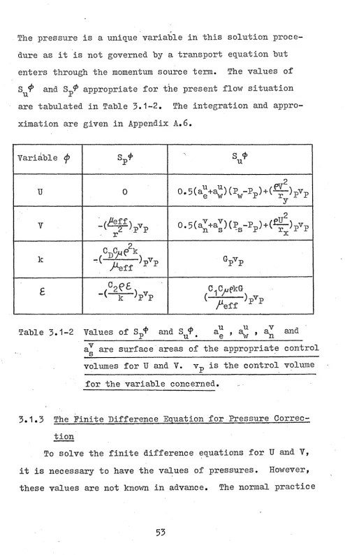
3.1.2 The General Expression of the
Finite Difference Equation 46
3.1.3 The Finite Difference Equation
for Pressure Correction 53
3.2 The Solution of the Finite Difference
Equation ^ 56
I 3.3 The Overall Procedure of Solution 59
Chapter 4 The Computer Model 62
4.1 Introduction 62
4.2 The Basic Structure of the Computer
Program . 6 2
4.3 The Simulation of Various Flow
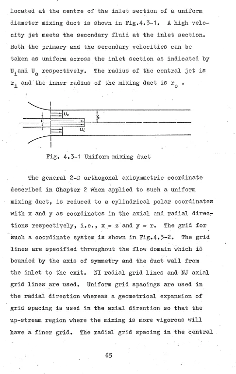
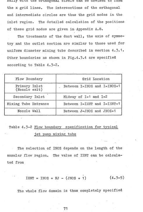
Components - 64
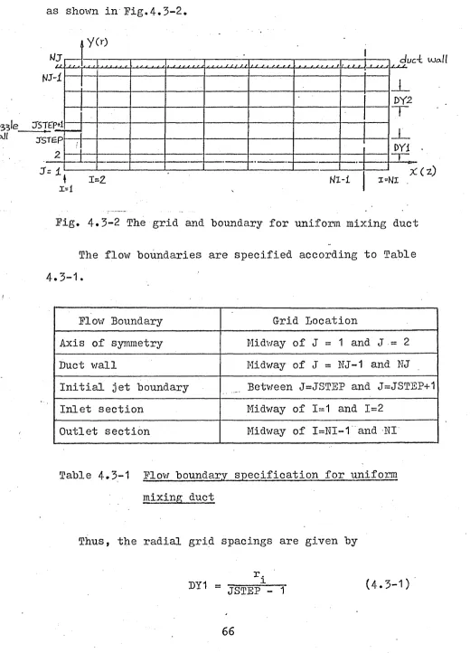
4.3.1 Uniform Mixing Duct 64
4.3*2 Typical Jet Pump Mixing Tube
Including Secondary Inlet Region 67
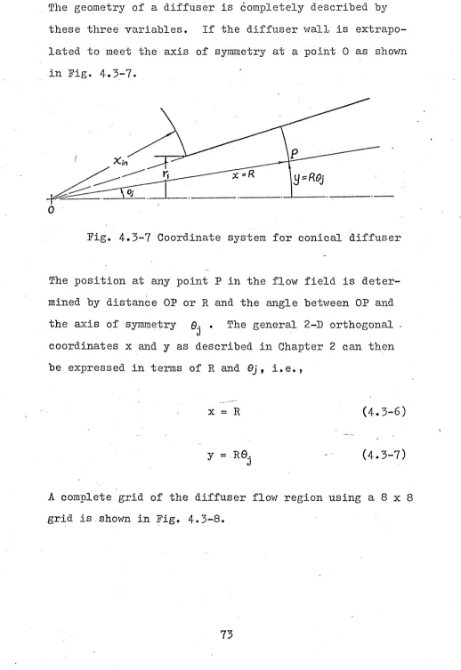
4.3.3 Conical Diffuser 72
Chapter 5 Flow Prediction 76
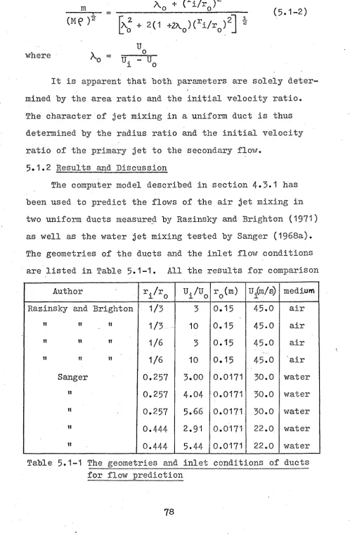
5.1 Flow in Uniform Diameter Mixing Tube 76
5.1.1 Introduction 76
5.1.2 Results and Discussion 78
5.2 Flow in Typical Mixing Tube Including
Secondary Inlet Region - 98
5.2.1 Introduction 98
5.2.2 Results and Discussion 99
5.3 Flow in a Conical Diffuser 107
5.3.1 Introduction 107
5.3.2 Results and Discussion 110
5.4 The Prediction of Overall Performance .
of Typical Jet Pump 114
5.4.1 Introduction 114
5.4.2 The Procedure of Calculating the
Overall Performance 117
I M S .
Chapter 6 Experimental Investigation 123
6.1 Introduction 123
6.2 The Jet Pump Test Rig 125
6.2.1 The Plow Circuit 125
6.2.2 The Components of the Test Pump 128
6.3 The laser Doppler Anemometry 136
6.3.1 The Measurement of Turbulent Plow 136 6.3.2 The Basic Principles of L.D.A. 137
6.3.3 The Optical Systems 140
6.3.4 Methods for Frequency Signal
Processing 145
I 6.3.5 Signal Quality 148
6.3.6 Frequency Shift 153
6 . 4 The Measurement of Mean and Fluctuating
Velocities Using L.D.A. 154
6.4.1 The Components of the Laser
Doppler Anemometer 154
6.4.2 The Measurement of Three Orthogonal Velocity Components in a Circular
Mixing Tube - 160
6.4.3 Experimental Procedure 177
6.4.4 The Limitation of L.D.A. and Design Criteria of the Optical
Components 179
6.5 Results and Discussion 183
6.5.1 L.D.A. Experimental Results 183
6.5.2 Comparison of L.D.A. Measurement
with Prediction 194
6.5.3 Discussion 197
6.6 Measurement of Static Pressure in
Mixing Tube and Diffuser 204
Chapter 7 Application of the Computer Model for
Jet Pump Design ■ , 209
7.1 Performance Prediction of Any Proposed
Design 209
7.2 Effect of Geometry on Jet Pump
. Performance 212
7.2.1 The Influence of Diameter Ratio 212 7.2.2 The Influence of Mixing Tube
Length 215
7.2.3 The Influence of Diffuser Included
Angle 218
7.2.4 The Effect of Nozzle Exit to
Mixing Throat Spacing 221
7.3 An Optimizing Procedure for Jet Pump
Design 224
Chapter 8
8* 1
8*2
Appendix A
A.1
A. 2
/
A* 3
A* 4
A* 5
A* 6
A. 7
A.8
j A. 9
Appendix B
References
Page
Conclusions and Suggestions for
Future Research 227
Conclusions 227
Suggestions for Further Research 230
One-Pimensional Theory of Jet Pumps,
Gosline and 0 *Brien(1934) 232
Momentum Integral Method of P.G.Hill
for Axisymmetric Ducted Jets 236
Derivation of Momentum Equation for
a Two-Dimensional Axisymmetric Plow 243
Derivation of k~Production Terms 247
Derivation of the General Finite
Difference Equation for cj> 249
Linearization of Source Terms 255
Derivation of the Finite Difference
Equation for P' 259
i Calculation of Orthogonal Grid in the
Secondary Inlet Region of Jet Pump 262
Inlet Conditions for Turbulent Kinetic
Energv k and Length Scale 1 267a
Listing of Computer Programs 268
ACKNOWLEDGEMENTS
I should like to thank my supervisor, Mr. D.R. Croft, for his guidance and generous help throughout the project. I should also like- to thank my second supervisor, Dr. M.J. Denman, for many helpful suggestions and comments on the experimental aspect of this project and the presentation of this thesis. My thanks are also due to Dr. P.D. Williams for his advice and encouragement in the early stages of
this work.
There are many staff in the Department of Mechanical and Production Engineering and the Department of Computer Services to whom my thanks are also due but I should
particularly like to mention Mr. D. Allen and Mr. R. Wilson for their assistance and contribution in the construction of the experimental rig.
I am also in debt to Mr. I. Rothwell of B.I.R.A.L. for the loan of a TSI tracker and several useful .discussions.
The work reported in this thesis was carried out during the tenure of a LEA research assistantship provided by the Sheffield City Polytechnic , without such financial support this work would not have been possible.
Finally, I should like to thank my wife for her continuing patience and help in the preparation of this thesis; and to my parents, who, from the other side of the world, consistently give me encouragement and moral support during my pursual of this work.
S. N. TAY
V
DECLARATION
Apart from the references cited, this thesis is
the original work of the author.
Some of the computer predicted results have been
used in a joint paper ‘Numerical Analysis of Jet Pump
F l o w s 1 published by the author and his supervisors at
the First International Conference on Numerical Methods
in Laminar and Turbulent flow held at the University
SUMMARY
As an.aid to jet pump design and performance analysis,
a theoretical investigation oh turbulent confined jet m i x
ing in a non-uniform axisymmetric duct typically used in
jet pumps and ejectors has been undertaken. A so-called
Prandtl-Kolmogorov two-equation turbulence model, with
turbulent kinetic energy k and turbulent energy dissipation
rate £ as the two parameters, is incorporated into the time-mean lTavier-Stokes equations to form a complete set
of partial differential equations which describes the
turbulent flow mathematically* The equations are solved
numerically via a primitive pressure-velocity
finite-difference procedure using a digital computer. The
time-mean static pressure, velocities, turbulent kinetic energy
and dissipation rate are predicted directly throughout the
whole flow field.
To validate the computer model, predicted time-mean •
static pressure and velocity as well as turbulent shear
stress for flow in a uniform bore mixing tube are compared
with the published results. The method is then extended
to predict flows in conical diffusers and typical jet
pumps. The predictions are also compared with the availa
ble experimental data.
A laser Doppler anemometer is used to measure the
mean and fluctuating velocities of water jet mixing in a
nozzle. The measured data which enable turbulent kinetic
energy to be evaluated, are compared with the computer
predictions to further consolidate the theoretical model.
Finally, the computer model is used to predict the
performance of a proposed jet pump and to investigate the
influence of various geometrical parameters on jet pump
performance. The capability of the computer model as
a useful design tool is also demonstrated via an optimi
zation procedure to give the optimum geometry for a given
NOMENCLATURE
The symbols are explained as they are introduced
throughout the thesis. Inevitably, some of the symbols
are used to represent more than one quantity. Unless
otherwise stated, the symbols will have the following
meanings.
Symbol
u v a ,a
aa’V cj’d;
j
o v o z
CD
c ,c ,c ,c
e9 w* n* s
c t
OjJL
D ,D ,D ,D e 9 w . n s
d
E
F
f
Meaning
Coefficients in the general difference equation
Surface areas of control volumes for U and V
Coefficients of the general algebraic equation for (f> in tri-diagonal matrix form
Constants in the source terms for turbulent energy dissipation S
Constant in the source term for turbulent kinetic energy
Coefficients in the convective terms of the difference equation
Craya-Curtet Number for confined jet flow
A constant in the equation for turbulent viscosity
Velocity of light
Coefficients in the diffusive terms of the difference equation
Diameter
A function of wall roughness in the logarithmic velocity distribution near the wall
Force
Doppler frequency
Turbulent energy production term
Total head
Incident angle of a light beam
Turbulent kinetic energy
Unit vector
Roughness parameter of a wall
Length in general or length scale in the turbulence models
Mixing length in Prandtl*s model
Plow ratio of a jet pump
Mass flow rate
Head ratio of a jet pump
Time-mean static pressure
Instantaneous and fluctuating static pressures
Primary and secondary flow rates of a jet pump
Radii of curvature of the nozzle wall and inlet duct wall respectively; also refer to inner and outer pipe radii in Chapter 6
-Reynolds number
Distance of a point from the axis of symmetry; also represents refractive angle in Chapter 6
Radii of the central jet and mixing duct for an uniform mixing duct
Radii of curvature for x and y surfaces respectively
Source term in the differental equation for <j>
Spacing.between nozzle exit and mixing tube inlet
Time in general; also thickness of a perspex wall in Chapter 6
Time-mean velocities in the x and y directions
Area-mean velocity of a duct
Instantaneous velocities in x and y directions
Fluctuating velocity components in three orthogonal directions
Turbulent velocity
Velocity vector
Streamwise and cross-stream coordinates for a general 2-D orthogonal axisymmetric coordinate system
2-D Cartesian coordinates
A turbulent quantity, km ln where m , n are constants; also represents the axial
direction of cylindrical polar coordinates
Angle between the axis of symmetry and direction x
Efficiency; also represents refractive index in Chapter 6
Diffuser included angle
Wave length of light
Laminar, turbulent and effective viscosi ties of the fluid
Density
Turbulent Prandtl/Schmidt numbers for k and £
Turbulent energy dissipation rate
Shear stress
Kinematic viscosity
JO von Karman constant in the logarithmic velocity distribution
Cp Beam intersecting angle
Subscripts
0 Mixing tube inlet section
1 Diffuser inlet section
a Quantity measured in air
c Centre-line value
d , Diffuser
e Entrained quantity
i Refers to inner in general; also refers
to incident beam in Chapter 6
in Inlet condition
D Primary jet
E,S,E,W Pertaining to neighbouring nodes which
lie respectively north, south, east and west of node P
n Hozzle exit
n,s,e,w Pertaining to the four sides of the
control volume surrounding node P
o Outer
P Pertaining to node P
p Quantity measured in perspex wall
s Secondary inlet section; also refers to
scattered beam in Chapter 6
t Mixing tube
w Quantity measured in water
x Refers to section at a distance x down
INTRODUCTION
Confined jet mixing is a fundamental fluid flow
phenomenon of practical engineering importance. It is
concerned with the mixing of a high velocity jet with a
slow-moving fluid stream in a duct. The design of many
devices such as jet pumps and ejectors, gas turbine
combustors, gas burners, etc., are all benefited from
the understanding of the mechanism of such flow. Despite
the wide application of confined jet mixing, the subject
received relatively little attention in' the past as com
pared with free jet flow or other boundary layer flows.
The present study is mainly aimed at confined jet mixing
related to jet pump design and performance analysis.
Jet pumps and ejectors are simple pumping devices
directly derived from the principle of confined jet
mixing. When a high velocity jet ejects into a mixing
chamber, the slow-moving adjacent fluid is dragged along .
in the jet direction. The mixing between the driving and
entrained fluid results in momentum transfer from the
high velocity driving jet to the low speed entrained
fluid. It is obvious that the increase in velocity in
the entrained fluid is achieved at the expense of the
energy of the driving j et.
, Unlike other pumping devices such as positive dis
placement, centrifugal or rotary pumps, a jet pump does
not require any moving part. Its working principle is
based on a purely fluid dynamic phenomenon. Do mechanical
energy is being used to increase the energy of the entrained
fluid. The advantages of such a primitive device are its
simplicity, reliability, absence of moving parts, and
cheapness.
Jet pumps are being used in many areas, such as
process industries; SfOL aircraft augmentation and
space-oriented systems; recirculation devices in nuclear reactors;
and more common, in deep-well pumping, booster pumping as
well as dredging and priming devices. Because of their-low
cost and easily replaceable nature, jet pumps are especially
suitable for pumping hostile fluids such as slurry which
might be harmful to other expensive pumps.
A typical jet pump consists essentially of a primary
nozzle, a suction chamber, a mixing tube and a diffuser
as shown in Big.0-1. The nozzle and the suction chamber
are connected to the driving line and suction line respec
tively. The two fluids undergo turbulent mixing in a
mixing tube and the combined fluids then pass through a
diffuser which serves as a pressure head recovery device;
The relevant geometries and flow conditions are also
indicated in the diagram.
The four fundamental parameters used for jet pump
design and performance analysis are usually presented in
non-dimensional forms. These are: . . .
v (i) the ratio of the entrained flow rate to the
(ii) the ratio of total head gained by the entrained
fluid to total head lost by the primary fluid,
known as the head ratio N;
H d - H s
H d - H d
(iii) the area ratio of nozzle to mixing tube, R;
R - ( ^ ) 2
and (iv) the efficiency , which is equivalent to the
output power divided by the net input power
Q2 (Ha “ Hs )
r ™
driving q2 line
W;
suction chamber
nozzle
diffuser entrance mixing tube
region
suction line
Fig,0-1 Typical Jet Pump Configuration
Other geometrical variables of significant importance
on performance and design are mixing tube length 1^,
nozzle to mixing tube spacing s and diffuser included
angle Q . Wall profiles of the secondary entrance region may also have some influence over the performance.
Although jet pumps have- been the subject of extensive
experimental studies, very few investigations have dealt
with the basic flow behaviour. The inadequacy of theore
tical and experimental studies on confined jet mixing has
led to a situation whereby the designs of jet pumps and
ejectors in the past have largely relied on empirical
data obtained from model pump testing. Performance
prediction is unreliable as it varies for each individual
design. Owing to the large number of geometrical parame
ters involved, the previous research has not been able to
provide consistent design recommendations. There is also
a lack of a satisfactory explaination on the limitation of
jet pump performance such as low head rise, low
entrain-ment ratio or low efficiency.
This thesis reports the research work carried out
by the author. The thesis can be divided into three
parts:
(i) The development of a set of computer models
which predict flows in (a) the mixing*tube'
region; (b) the entrance region; and (c) the
diffuser region of a typical jet pump device.
(ii) Experimental studies of turbulent confined jet
mixing using a laser Doppler anemometer for the
measurements of mean and fluctuating velocities,
(iii) The application of the computer prediction tech
of jet pumps.
The present theoretical approach, unlike the previous
analytical methods which relied on large amount of empiri
cal input data, is to incorporate the Prandtl-Kolmogorov
two equation k~ £ turbulence model into the time-mean
Navier Stokes equations to form a set of partial differ
ential equations. The equations, which are elliptic in
character, are solved numerically by a finite difference
procedure using a semi-implicit line by line method to
gether with a tri-diagonal matrix algorithm. The primitive
variables,pressure and velocity are solved directly rather
than using the vorticity-stream function approach.
The flows in the entrance region, mixing tube and
diffuser are solved through using similar but separate
computer programs. This enables the use of the most
appropriate co-ordinates system for each flow configura
tion as well as avoids the excessive storage requirement
on the computer. The computed time-mean velocity,
^irbu-lent shear stress and static pressure distributions in
these flow regions are compared with the existing experi
mental results from various sources.
The laser Doppler anemometry (L.D.A,) technique is
employed to measure the time-mean and fluctuating r.m.s.
velocities in the mixing tube where turbulent mixing of
two co-axial jet streams takes place. The turbulent
kinetic energy in the mixing tube is calculated from
the three orthogonal r.m.s. velocities. The measured
time-mean velocity and turbulent kinetic energy are then
compared with the computer prediction. The accuracy and
limitation of using the L.D.A. for the measurement of turbu
lent water jet mixing are also discussed.
Finally, the computer programs are used to predict
pressure and velocity fields for various geometrical
combinations, i.e. area ratio, nozzle spacing, mixing
tube length and diffuser included angle. The effect of
varying any geometrical parameter on jet pump performance
is also studied. The final development computer model
provides a useful tool for jet pump and ejector design.
The designer needs only to specify geometry and required
flow ratio in order to obtain information such as pressure
rise, thrust augmentation, and efficiency. An optimiza
tion procedure is also developed to enable the designer
to obtain optimum geometrical combination with best
CHAPTER 1
PREVIOUS RELATED STUDIES
1.1 Historical Development of the Theory of Jet Pumps
The use of water jet pumps has existed for more than
a hundred years. The first known application of a water
jet pump was made hy James Thomson in 1852. Since then,
numerous theoretical and experimental studies on jet pump
design and performance have been carried out. The theory
of pumping through the mixing of two jet streams was first
developed by J. M. Rankine (1870) based on the one
dimensional continuity and momentum equations. This
concept of analysis is still widely used at the present
time, with little or no addition to improve the prediction.
Gosline et al (1934) applied the one-dimensional
concept to derive the head ratio and efficiency for water
jet pumps with cylindrical mixing chambers. The details
of the derivation are described in Appendix A . 1. Reasonable
prediction of performance was obtained by the authors
using the analysis but only by assuming empirical loss
coefficients for the driving line, suction line, mixing
tube and diffuser. The treatment is a simple method used
in general fluid flow analysis which ignores the details
of the mechanism by which the two streams mix with one
another. No generality can be claimed by such an analysis
as its prediction is based on the experimental-determined
loss-coefficients on specific jet pumps. However, owing
to its simplicity, the method was employed by many other
workers, including Cunningham et al (1954-)9 Mueller (1964)?
Reddy et al (1968), and Sanger (1968a, 1971) etc. An
attempt was made by Mueller tq improve the prediction
using two frictional loss-coefficients to account for
the developing and developed flows in the mixing tube,
but the modified version did not improve the prediction
(Sander, 1968a). A method of designing liquid-to-liquid
jet pumps using a simple computer program based on the
one-dimensional analysis was developed by Sanger (1971)*
Cunningham (1975) also derived a modified head ratio
expression which took into account the ’jet l o s s 1 due to
the space between the nozzle and the mixing tube. It was
found that the improvement in prediction was only marginal
and not applicable to all cases.
Two-dimensional analysis of axisymmetric confined
jet mixing using momentum integral methods has been carried
out by several researchers. The earlier works of this
kind can be found in Curtet (1958), and Dealy (1964).
More comprehensive theoretical analysis was done by
P. G-. Hill (1965, 1967). After assuming a virtual source
located at nozzle exit plane, Hill divided the downstream
into three distinct flow regions, namely, potential outer
flow region, recirculation region and wall-jet interaction
region as shown in Pig. 1.1-1. He was able to predict the
mean velocity and pressure distributions using empirical
data of velocity and turbulent shear stress distribution
to confined jet flow with relatively small nozzle diameter
as compared with that of mixing tube. The main deficiency
was thus its inability to predict the flov; behaviour in
the potential core region for -high nozzle to mixing tube
diameter ratios frequently used in jet pumps and ejectors.
The analysis is fully described in Appendix A.2.
Nozzle Mixing Duct
A : Potential outer flov; region B : Recirculation region
C : Wall-jet interaction region
Fig.1.1-1 Plow Regimes of H i l l Ts (1965) Analysis
The development of momentum integral method was
carried a step forward by B. J. Hill (1971> 1973)* He
extended the analysis to include the potential core region
and used empirical data directly derived from jet pump
measurement. The major shortcoming of the integral method
is the necessity to use a large amount of empirical input
data. The accuracy of analysis thus depends on the range
of geometrical and flow conditions under which the empiri-'
cal data was evaluated.
More recent theoretical development of jet pump and
confined jet mixing is focused on solving turbulent
port equations using finite difference procedures,
Hedges et al (1972, 1974) devised a finite difference
model based on the conservation equations and Prandtl's
mixing length hypothesis to predict the mean velocity
and pressure distributions. Pope (1972) also used the
Patankar-Spalding finite difference procedure (1967)
incorporating a mixing-length hypothesis to solve for
the mean flow behaviour. However, no prediction of
turbulent shear stress or other turbulent quantity is
reported. It is clear that in order to study the
turbulent nature of confined jet mixing and to .predict
jet pump flow more reliably, a more advanced turbulence
model must be employed. .
1.2 Numerical Methods for Predicting Turbulent Plows
, In.the past twenty years, following the development
and application of high speed digital computers, tremen
dous amount of research works have been devoted to the
field of numerical methods for predicting turbulent
flows. To summarized the various methods being used
and published, it would require a relatively long
chapter. However, despite the great variety of methods,
it is possible to divide them, according to the computa
tional procedures involved, into two main categories,
i . e . ,(i)integral methods, and (ii) finite-difference
methods.
1.2.1 The Integral Methods
from experimental measurements, such as the shape of the
velocity profile, the shear stress distribution and skin
friction coefficient for the solid wall, to incorporate
into the integral equations of conservation* The result
ing set of ordinary differential equations are then solved
by some appropriate numerical integration procedures such
as Runge-ICutta method. The applications of these methods
to predict turbulent boundary layer flows were reported
by Truckenbrodt (1952), Head (1960), Escudier and Spalding
(1965) and Escudier and Hicoll (1966). Curtet (1958),
Mikhail (I960), Eealy (1964), Hill (1965), Exley and
Brighton (1971) and Hill (1975) have applied the integral
methods to predict confined jet flows. The detail des
cription of H i l l ’s (1965) approach which is a typical
integral method is included in Appendix A.2.
The widespread use of integral methods lies on the
fact that much less computer time is required as compared
with the finite difference methods. However, the inte
gral methods are lacking in. generality and large amount
of empirical information is required. In order to
predict different flow regions, various empirical forms
for velocity profile and shear stress distribution to
suit various'flow components are therefore needed a s #
input data to obtain reasonable result. In view of
these deficiencies, the search for more general methods
to predict turbulent flows through solving the governing
partial differential equations numerically was the m a i n
concern in this field for the past two decades.
1*2*2 The ITin.ite Difference Methods
The solving of partial differential equations of
mass, momentums and other variables for turbulent flows
could only be achieved if the flow could be treated as
obeying the Newton*s viscosity law with an appropriate
effective viscosity* Such concept of 11 turbulent” or
"eddy” viscosity was first introduced by Boussinesq in
1877* He proposed that the effective turbulent shear
stress Tt could be replaced by the product of the
time-mean velocity gradient and the turbulent viscosity p - t
? t = A I ? (1-2" 1)
where U is the time-mean velocity and y is the cross
stream distance.
The introduction of the turbulent viscosity concept
does not solve the problem completely but at least
provides a basis for turbulence modelling. The main
task left behind is to express the turbulent viscosity
in terms of quantities which can be determined, either
by solving some algebraic equations or partial differen
tial equations.
Prandtl's mixing length hypothesis Based on the analogy
to the kinetic theory of gases, i.e., the viscosity is
proportioned, to the product of the density, the r.m.s.
velocity of the molecules and the mean free-path,
the turbulent velocity u^ and a length 1 called mixing
length,
/a t = e 1m u fc (1.2-2)
He then further proposed that the turbulent velocity was
equal to the mixing length 1 times the longitudinal
time-mean velocity gradient,
(1.2-3) lu ~ 1™t m ^2
^y
Thus, the complete mixing-1 ength hypothesis will
have the following mathematical relationship
_ -i 2
M t “ P m (1.2-4)
Prandtl went on to suggest that 1 was proportional to
the distance from the nearest wall. In the case of
free turbulent flows, Prandtl made an assumption that
■1 was proportional to the width of the turbulent
mixing zone and thus only dependent upon the distance
along the main flow direction but not the lateral
direction.
P r a n d t l fs m i x i n g ‘length hypothesis was incorporated
into the partial differential equations of conservation
for boundary layer flows and solved numerically by
Patahkar and Spalding (1967). The predictions of
time-mean velocity distribution in free jets and in
turbulent flow on flat-plate were found to agree reasona
bly well with measurements. The method was also extended
to predict the temperature, mass concentration in boundary
layer flows by the same authors. Application of the method
to predict mean flow behaviour of jet pump was reported
by Pope (1972).
The main shortcomings of the mixing length hypothesis
are (1) turbulent viscosity is zero at those location
~\TJ
where — = 0 whereas experiments have shown otherwise;
(2) no account is taken of the processes of convection
and diffusion of turbulence in which the local turbulent
velocity is affected by the neighbouring fluids.
One-equation models of turbulence The shortcomings of
the mixing length hypothesis was overcome by the proposals
of Prandtl (1945) and Kolmogorov (1942) who independently
suggested that the turbulent viscosity was proportional
to the square root of the turbulent kinetic energy k. as
/it ( 1 . 2 - 5 )
where k = M u ’^ .+ .v1^ + w 1^) . .
u 1, v* and w* are the three orthogonal r.m.s. velocities,
1 is a length scale and k is to be determined from a.
transport equation. Prandtl and Kolmogorov derived the
lc-transport equation separately from the Navier-Stokes
equations. The final approximated form of the k-equation
can then be solved simultaneously with the momentum and
to predict the turbulent flow in a sudden enlarged pipe
and by Wolfshtein (1 9 6 8) in predicting the impinge jet flow* Pun and Spalding (1967) also succeeded in apply
ing the similar model to predict turbulent confined jet
mixing in cylindrical combustion chamber*
Instead of using the concept of turbulent viscosity,
Bradshaw et al (1967) assumed that the turbulent shear
stress is proportional to a variable called turbulent
energy k 1,
T t = CflC
where C is a constant* They derived a transport equation
for k 1 which was then solved together with other conser vation equations. Satisfactory predictions were obtained
for a number of external wall boundary layer flows. Nee
and Kovasznay (1 9 6 9) also proposed that the kinematic turbulent viscosity should be determined directly by a
transport equation* All the above methods are always
referred to as. one-equation models of turbulence. The
major shortcoming of these models is that the length
scale 1 which always appeared in the transport equation is needed to be prescribed algebraically. A precise pres
cription of 1 is, however, rarely possible except for boundary-layer flows*
Two-equation models of turbulence The deficiency of the
one-equa.tion models has led to the search for more compe
tent models to be able to predict turbulent flows w i t h
out prescribing the length scale algebraically. Such
models require that another variable related to the
length scale should be determined by an additional
transport equation and can thus be referred to as
two-equation models. Perhaps IComogorov (1942) was the first
person to propose the idea of two-equation model. In
1942, he suggested that the turbulent viscosity could
be determined by the turbulent kinetic energy k and the
characteristic frequency of energy-containing motions f
so that
A t = f T (1.2-6)
Both k and f should be determined from separate differen
tial transport equations. Comparing equation (1.2-6)
with equation (1.2-5), it can easily be seen that
IComo-gorov actually chose k 2/l as his second dependent variable.
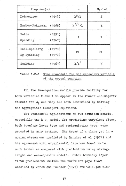
Prom then onwards, many authors have proposed various
two-equation models using different dependent variables *
among them are Rotta(1951) and Spalding (1967) who used 3/2 k and 1; Harlow and Nakayama (1968) who used k and k / 1 Rotta (1971)> Ng and Spalding '(1972) who used k and kl
and Spalding (1969) who used k and k/l^. It is apparent
that the difference among various two-equation models is
the choice of the second dependent variable to determine
the length scale. If the second variable is designated by
z = km ln with m and n being constants, a summary of various
Proposer(s) z Symbol
Kolmogorov 1942) . ls^/l f
I-Iarl ow-Rakayama 1 9 6 8) k 5/2/l £
Rotta
Spalding
1951)
1967)
1 l
Rodi-Spalding
Kg-Spaiding
1970)
1972)
kl kl
Spalding 1969) k/1 2 W
Table 1*2-1 Some proposals for the .dependent variable
of the second equation
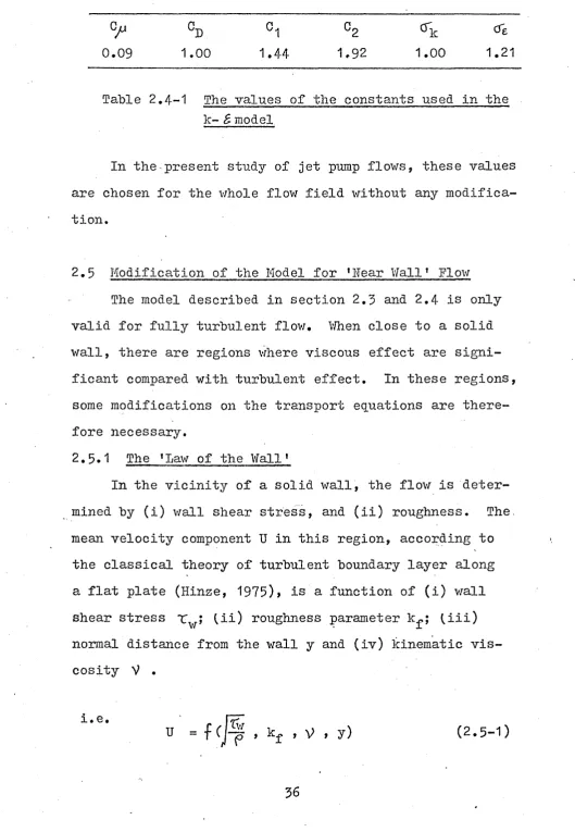
All the two-equation models provide facility for
both variables k and 1 to appear in the Prandtl-Kolmogorov
formula for and they are both determined by solving
the appropriate transport equations.
The successful applications of two-equation models,
especially the k - £. model, for predicting turbulent flows,
both boundary layer type and recirculating type, were
reported by many authors. The decay of a plane jet in a
moving stream was predicted by Launder et al (1972) and
the agreement with experimental data was found to be
much better as compared with predictions using
mixing-length and one-equation models. Other boundary layer
flows predictions include the turbulent pipe flows
obtained by Jones and Launder (1973) and wall-jet flow
[image:33.614.25.545.23.794.2]predicted by Sharma (1972). In recirculating flows,
prediction of film cooling was obtained by Matthews and
Whitelaw (1 9 7 1)> cylindrical furnace flow was predicted by Elghobashi and Pun (1974) and forced cavity flow was
reported by Nielson (1973).
Multi-equation models of turbulence Other turbulence
models being proposed include the three-equation model of
Hanjalic (1970) who used k, £ and u ’v*" as dependent
variables and the five-equation model of Paly and Harlow
— — 77
(1 9 7 0) in which the normal turbulent stresses u* , v ! and w* together with u ^ v1 and £ are determined by five differential transport equations* However, few successful
prediction based on the multi-equation models has been
reported, This suggests that a model of such complexity
is not.yet-well established for general application.
The solution procedures employed Almost all the early
solution procedures for calculating turbulent flows
using finite-difference method were based on the.computer
code developed by Patankar and Spalding (1967) and
Gosman et al (1969). The former solved parabolic equations
in boundary layer flows and the later solved elliptic
equations in recirculating flows. Both procedures employ
ed the stream function-vorticity approach which solved the
stream-function and vorticity together with the turbulent
parameters and then transformed back to time-mean velocities
and pressure. New solution procedures which solved the
primitive variables,velocities and pressure,were develop
They were widely tested in many flow predictions as
reported by G-osman and Pan (1974) and Pun and Spalding
(1976).
1.3 Previous Experimental Studies
1.3.1 Experimental Studies on Confined Jet Mixing
The early experimental studies of confined jet
mixing were mainly concerned with mean'.flow, behaviour.
The centre-line velocity, the static pressure and the
velocity profiles were the main interests to many
researchers. Measurements of centre-line velocity
decay and velocity profiles across various sections in
uniform duct were first obtained by Eorstall and Shapiro
(1950). Static pressure along the duct wall and velocity
profiles were measured by Helmbold et al (1954) who used
both uniform and non-uniform mixing ducts. Other similar
measurements- of mean flow behaviour include those made by
Mikhail (1960), Becker, Hottel and Williams (1962), Dealy
(1964), etc., all using Pitot static tube for their velo
city measurements.
Turbulent fluctuating velocities in both longitudinal
and radial direction of a confined jet flow were first
measured by Curtet and Ricou (1964) using a
constant-temperature hot-wire anemometer. The most complete
measurement of confined jet mixing to date was probably
done by Razinsky and Brighton (1971) who measured the
centre-line velocity, the wall static pressure, the
velocity profiles, the longitudinal r.m.s. velocity as
well as the Reynolds stress. The mean velocity was
measured hy a Pitot static tube and the turbulent quanti
ties were measured by a constant-temperature hot-wire
anemometer. All these works have contributed a great
deal to the understanding of the mixing behaviour in
ducts.
1 . 5 . 2 Bxperimenta.1 Studies on Jet Pumps and Bjectors
Large amounts of literature on experimental studies
of jet pumps' and ejectors have been accumulated in the
past fifty years. Most of the literature is summarised
in a BHRA Review compiled by Bonnington and King (1972).
The earlier works on jet pumps are mainly concerned with
performance tests and pressure rise measurement along
the duct wall. Typical works of such are those of G-osline
et al (1 9 3 4), Keenan et al (1942), Polsom (1948) and Kastner et al (1950).
Many experimental investigations have also been
devoted to various geometrical effects on jet pump
performance. G-osline et a l (-1934), Vogel (1956),
Mueller (1964) and Hansen et al (1965) carried out
experimental tests and recommended 'a mixing tube
length ranging from 3 . 5 to 8 . 0 diameters for optimum performance. As for the effect of nozzle to mixing
tube spacing, Schulz (1952) established that the
optimum spacing lie between 1 and 2 nozzle diameters whereas Hansen et al (1965) recommended a value between
0.8 and 1.4. -Schulz (1958) and Mueller (1964) also
having the secondary flow inlet in the shape of a round
ed bell mouth. The diffuser angle is another geometrical
variable which many workers have made considerable experi
mental studies in order to give a recommendation to achieve
a good performance. Mueller (1964) recommended a 5°
diffuser included angle for best efficiency whereas an
8° included angle was proposed by Vogel (1956). It is clear that although many efforts have been devoted to the
investigation of geometrical effects on jet pump perform
ance, no consistent recommendation of optimum geometrical
configuration has been made. The facts that a large number
of geometrical variables are involved and their interre
lated effects on the flow behaviour in mixing tube and
diffuser make it extremely difficult to generalize the
problem.
Experimental studies of several low-area-ratio water
jet pumps were carried out by Sanger (1968a, 1968b, 1970).
Static pressure and efficiency were obtained for two' area
ratios of 0.066 and 0.197. . T h e mixing tube lengths used
were 7 . 2 5 and 5 . 6 6 diameters whereas nozzle spacing rang ing from 0 to 2.9 tube diameters. It was observed that
the efficiency for the shorter mixing tube pump was about
2% higher for both area ratios which suggested that
for these area ratios, mixing tube length, between 5 and 6 diameters was sufficient for optimum mixing. -However, it was concluded by the author that because of the inter
dependence among, the various geometrical parameters, no
optimum geometries can be established for all jet pumps.
Other experimental studies on jet pumps are concerned
with applications of jet pump devices under various operat
ing conditions, cavitation studies and using jet pumps to
pump a dissimilar fluid*
1.4 Previous Applications of Laser Doppler Anemometry on
Related Plow Measurements
I The first successful application of laser Doppler
anemometry to.the measurement of fluid velocity can he
attributed to Yeh and Cummins (1964)* In their pioneering
work, they measured the velocity in a fully developed
laminar pipe flow of water. The technique was later
applied to turbulent water flows by others including
Goldstein and Hagen (1967)» Welch and Tomme (1967)? etc.
The measurement of turbulent air flow was carried out by ...
Lewis, Foreman,. Watson and Thornton (1968) and Haffaker,
Puller and Lawrence (1969). The technique has been used,
for example, by Durst and Whitelaw (1971) to measure the .
mean and fluctuating velocities of an axisymmetric air
jet; by Helling and Whit el aw (1973) to measiire the three
orthogonal components of mean and r.m.s. fluctuating
velocities of a rectangular water channel flow* Measure
ments' of turbulent shear stresses in pipe flow using two
trackers and a correlator were obtained by Bourke et al
(1971) and Morton and Clark (1971)*
More recently, laser. Doppler anemometry has been
applied to measure some highly turbulent flows using
(1 9 7 4) carried out measurement of mean and fluctuating velocities downstream of a square flow obstacle with
turbulent intensity up to 5 0 % , Baker (1974) reported the
measurement of three orthogonal r.m.s. velocities in the
fully developed region of a turbulent jet. The mean and
fluctuating velocities downstream of an annular jet with
substantial recirculation were measured by Durao and
VJhitelaw (1974). It is obvious that the laser Doppler
anemometry, although a rather new technique, will emerge
as a very powerful tool in the future fluid flow measure
ments.
CHAPTER 2
THE MATHEMATICAL MODEL
In this chapter, the partial differential equations
governing the basic lav/s of conservation of mass and
momentum for a incompressible viscous fluid are first
described. The equations, when apply to a turbulent
flow, require the additional terms to account for the
fluctuating components of the variables. A two-equation
k- £ turbulence model which provides informations for the
extra terms is incorporated into the time-mean differen
tial equations to form a complete mathematical model for
the two-dimensional axisymmetric turbulent flows. Appro
priate boundary, conditions which simulate the practical
jet pump situation in order to obtain realistic prediction
are discussed.
2.1 The Equations of Motion for an Incompressible Yiscous
Pluid
The derivation of the equations of motion based on
the basic laws of conservation are readily available in
many standard text books on fluid mechanics such as
Schlichting (1960) and Hinze (1975)• The equations,
according to Hinze (1975)? when expressed in a tensor
notation, using Cartesian coordinates takes the following
forms:
Continuity: ~ + ^ 7 j ~ 0 (2.1-1)
Momentum equation in x^-direction:
Du.
PdF = ^ x T ^ j i * Fi (2.1-2)
3 = 1, 2, 3
where ( f . . is the stress in the x.-direction operates in a
ji l
plane which is perpendicular to the direction x.. F. is
an external force per unit volume acting on the fluid
in x^-direction.
For an incompressible fluid,
- 2 - cT.. = _ + _2_ ■2>Xj 31 '^ x i b x..
equation (2.1-2) can be written as
' „ ( ^ i + H h ) d x.a
Du. ^ >u. ju.
-l ^ / < H 7 + Scf)
i ~ D L D i J
p — —i. ~
— _j.
\ Dt b x . b x . + F ± (2.1-3)
d = 1» 2, 3
where p is the static pressure and j x is the dynamic
viscosity of the fluid. Equations (2.1-1) and (2.1-3) are
usually referred to as the Havier-Stokes equations which
form the basis of the whole theory of viscous fluid mecha
nics.
2.2 The Need for Turbulence Modelling -- v •
The equations of motion described in section 2.1
are generally applicable to laminar flows but not turbu
lent flows. In brief, a turbulent flow is defined as an
irregular fluid motion in which the various quantities
show a random variation with time and space coordinates.
Turbulent flows can occur when fluids flow through
conduits (turbulent pipe flow), pass over solid bodies
(wake), or when neighbouring stream of the fluids with
different velocities pass over one another (jet mixing).
At present, one is unable to obtain solution for the
time-dependent turbulent flow field using existing computers.
Fortunately, it is possible to describe turbulent flow
with distinct average values of various quantities such
as velocity, pressure and temperature, etc. If a turbu
lent flow field is quasi-steady, averaging with respect to
time can be Lised. But for a homogeneous turbulent flow
field, averaging with respect to space is preferred. In
most of the engineering problems, time-averaged values
are more useful for engineers and designers.
The instantaneous values of velocity and pressure can
be written as
-u i = U i * -u i l (2.2-1)
and p «'P + p« (2.2-2)
where U. and P are the time-mean values and u . 1, p f are
1 i
the fluctuating values.
' The equations of motion for the average values in
turbulent flow were first derived by Osborne Reynolds.
He substituted the instantaneous values of u^ and p into
the equation (2.1-3) to give the following form.
DU. ^ -s ^U. ?>U._____ ____
p — 1 j. JS— n( — ~ ~— 1) - puJut ) V D t ‘Ox. *ax. / V2x. 7>x. } \ l D
1 J L J ^ «
+ P. (2.2-3)
l
Compare this equation with the original momentum equation
(2.1-3), it can he seen that the extra-terms - pu. ’u . ’ 1 J
are required to add to the viscous stresses in order
that the instantaneous variables can he substituted by
their time-mean values. Because Reynolds was the first
person to derive the equation for turbulent flow in this
form, the turbulent terms-p'u. !u a r e often called Rey-j- j
nolds stresses.
To solve equation (2,2-3), the terms - p u ^ ’u m u s t
be known. Since there is no direct way of knowing the
magnitude of these terms, a mathematical model to relate
effect with'known quantities is therefore required. Thus,
a model of turbulence, in the words of Launder and Spalding
(1 9 7 2) will !propose a set of equations which, when solved with the mean-flow equations, allows calculation of the
relevant correlations and so simulates the behaviour of
real fluid in important respects1.
2,3 The Differential Equations of Conservation Applied
to Two-Dimensional Axisymmetrical Flows
2,3*1 The Coordinate System
Before making any attempt to express any equation for
a particular flow configuration, an appropriate coordinates
system must be chosen. In this thesis, owing to the fact
that fluid flows take place at various flow components,
the most general two-dimensional orthogonal axisymmetrical
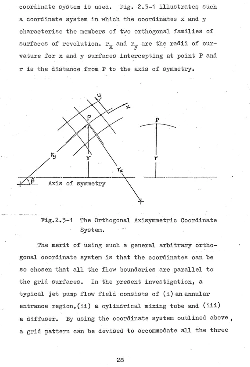
coordinate system is used. Fig. 2.3-1 illustrates such a coordinate system in which the coordinates x and y
characterise the members of two orthogonal families of
surfaces of revolution, r and r are the radii of
cur-x y
vature for x and y surfaces intercepting at point P and
r is the distance from P to the axis of symmetry.
Axis of symmetry
Fig.2.3-1 T h e .Orthogonal Axisymmetric Coordinate
System.
The merit of using such a general arbitrary ortho
gonal coordinate system is that the coordinates can be
so chosen that all the flow boundaries are parallel to
the grid surfaces. In the present investigation, a
typical jet pump flow field consists of (i) an annular
entrance region,(ii) a cylindrical mixing tube and (iii)
a diffuser. By using the coordinate system outlined above
[image:44.615.45.545.36.770.2]flow regions as shorn in F i g.20'3-2
mixing tube
Axis of symmetry secondary /
inlet primary
ini et
Fig.2*3-2 The coordinate system applied to jet pump
configuration
In general,' r . r and r are function of x and y< x y
In the uniform mixing tube region,
r = o° x
r - oo
y
r = y
In the diffuser region,
rx = 0 0 r = x + x
y
o
r = (x + x o )sin|6
(2.3-1)
(2.3-2)
where x Q and p are given in Figure 2.3-3 and their values
depend on the diffiiser included angle and the inlet diame
ter.
__
Axis of symmetry diffuser
inlet
Pig.2.3-3 Diffuser geometry
In the annular entrance region, explicit expressions for
rx , r^. and r are much more cumbersome. However, all the
variables x, y, r , r and r can conveniently be
calcula-x
y
ted in terms of Cartesian coordinates. Details of the
calculation will be illustrated in section 4.3.2. 2.3.2 The Differential Equations of Conservation
. The equations for conservation of mass and momentum,
when expressed in the general orthogonal x, y coordinate
system described above for a steady flow, will take the
following forms. __
The continuity equation,
Ie ( prTJ) + ^ (rrT) =
0 (2*5" 3)The momentum equation in x-direction,
■3/^ . 7 > , 3TJ'
where
Su = 1
r
dx^efflx^ * ay^efflx^
2yUeff(Usin|3 + Y c o s p )
. £ s d r
y
s m
f
(2.3-4)The momentum equation in y~direction;
^(piJrV) + ^ ( ?VrV) - ^ ( r ^ effg ) - J g r f r ^ f E )
¥ *
sT
QV 1 r
dU-^x^r /^eff dy^ + ^ r ^ / ^ e f f ^y^
2/ e f f ( U s i n /3 + Vcosp )
“ Is
is: r x
cos, (2.3-5)
where U, V, P are time-mean velocities and static pressure.
The full derivation of the momentum equations is given in
Appendix A.3.
The momentum equations are obtained by assuming that
the fluid is treated as obeying !Iewton!s viscosity lav/.
For a turbulent flow, jUq^ accounts for both viscous
stress and Reynolds stress. By comparing equation (2.3-4)
with equation (2.2-3)* one can write
OT. 3U. 7>U, 3U._____ ____
/ • e f f f e + ^ = / (:s q + ^ (2*3_6)
J d -1*
An appropriate model of turbulence is thus required to
relate the turbulent stresses - pu.* u .r to some i j
known quantities throughout the flow field.