On the accuracy of judgmental interventions on forecasting support systems

Lancaster University Management School

Working Paper

2005/022

On the accuracy of judgmental interventions on forecasting

support systems

Konstantinos Nikolopoulos, Robert Fildes, Paul Goodwin and

Michael Lawrence

The Department of Management Science

Lancaster University Management School

Lancaster LA1 4YX

UK

© Konstantinos Nikolopoulos, Robert Fildes, Paul Goodwin and Michael Lawrence All rights reserved. Short sections of text, not to exceed

two paragraphs, may be quoted without explicit permission, provided that full acknowledgement is given.

The LUMS Working Papers series can be accessed at http://www.lums.lancs.ac.uk/publications/

On the accuracy of judgmental interventions on Forecasting

Support Systems

Konstantinos Nikolopoulos

, Robert Fildes

, Paul Goodwin

,

Michael Lawrence

1 _{Department of Management Science, Lancaster University Management}

School, LA1 4YX, United Kingdom.

2 _{The Management School, University of Bath, Bath, BA2 7AY, United}

Kingdom.

3 _{School of Information Systems, Technology and Management, University of}

New South Wales, Sydney 2052, Australia

Working Paper

Abstract

Forecasting at the Stock Keeping Unit (SKU) disaggregate level in order to support operations management has proved a very difficult task. The levels of accuracy achieved have major consequences for companies at all levels in the supply chain; errors at each stage are amplified resulting in poor service and overly high inventory levels. In most companies, the size and complexity of the forecasting task necessitates the use of Forecasting Support Systems (FSS). The present study examines monthly demand data and forecasts for 44 fast moving, A-class, durable SKUs, collected from a major U.K. supplier. The company relies upon a FSS to produce baseline forecasts per SKU for each period. Final forecasts are produced at a later stage through the superimposition of judgments based on marketing intelligence gathered by the company forecasters. The benefits of the intervention are evaluated by comparing the actual sales both to system and final forecasts. The findings support the case that adjustments do improve accuracy, particularly under the condition that the adjustment is conservative, in the right direction, but does not overshoot. The question is how best to meet these conditions.

1. Introduction

Forecasting at the Stock Keeping Unit (SKU) level in order to support operations management has proved a very difficult task (Fildes et al. 2002, Fildes and Beard 1992). The levels of accuracy achieved have major consequences for companies at all levels in the supply chain; from retailer through to raw materials supplier. Errors at each stage are potentially amplified, resulting in poor service and overly high inventory levels, the so-called Bullwhip effect, (Lee et al. 1997). The forecasting problem is difficult due to the problematic nature of the data series. These data difficulties are compounded by the huge number of SKUs that need to be forecasted every period, often weekly or even daily, making complex forecasting methods usually inapplicable because of time and data constraints (Balkin and Ord 2000, Makridakis and Hibon 2000,).

In the majority of companies, because of the size and complexity of the forecasting task, it is impossible for all their SKUs to be tended individually by forecasting experts, necessitating the use of Forecasting Support Systems (FSS). The statistical forecasts (hereafter called the “system” forecasts), provide initial sales estimates which, for a number of key products, the forecaster is encouraged to amend, based on his/her knowledge of special events affecting the product (SKU) or the data (Fildes et al. 2005). This becomes the “final”forecast, a combination of a statistical forecast and managerial judgement (also referred to as marketing intelligence).

The present study aims to examine the accuracy of judgmental interventions in Forecasting Support SystemsWhy is this interesting? First of all because judgmental interventions are common in practise. There is evidence that managers like to adjust forecasts in order to retain a sense of personal ownership of them. Why is it important? Efficient forecasts are essential since there are major costs involved in the process; inaccurate forecasting leads to less profit as it results in either overstocking or lost sales.

months of available history. The company relies upon a FSS to produce system forecasts per SKU for each period. The forecasting method underneath the company’s FSS uses a selection routine including moving averages, single and Double Exponential Smoothing based on seasonally adjusted data (Gardner and Anderson, 1997). Final forecasts are produced at a later stage through the superimposition of judgments based on marketing intelligence by the company forecasters. In this study, the benefits of the intervention are evaluated by comparing the actual sales both to system and final forecasts.

This study is structured as follows. The next section reviews the relevant literature. Section three describes the data and is followed by an evaluation and a discussion of the key results. The last section presents the conclusions of this study as well as a roadmap for future research.

2. Demand Forecasting at SKU level

The strongest evidence that judgmental interventions can be effective when applied to SKU data comes from Mathews and Diamantopoulos with a series of contributions (1992, 1990, 1989, 1986) showing that judgmental “revision” improves accuracy even though some times only marginally. Their results were verified over a very large sample of more than 900 SKUs. The first study (1986) examined the improvement of judgmental interventions over only one period (quarter) and the outcome was that at least the revised forecasts were of lower variance. The longitudinal extension of this study came in the next study (1989) where data and forecasts over six consecutive quarters were examined. Stronger evidence was found of improvement in the forecasting process as a result of the judgmental interventions. The third study (1990) showed the effectiveness of forecast selection; the final study (1992), an examination of the relative performance of judgmentally revised versus non-revised forecasts, indicated that there were significant differences.

The most renowned of the studies of company data is the M2-competition, the second part of the famous Makridakis’ trilogy (Makridakis et al. 1982, 1993, Makridakis and Hibon 2000) where domain knowledge was available for all the series under consideration. The purpose of the M2-Competition was to determine the post sample accuracy of various forecasting methods. It was an empirical study organized in such a way as to avoid one of the major criticism of the earlier M-Competition, that forecasters in real situations can use additional information to improve the predictive accuracy of quantitative methods (Makridakis et al. 1993).

who participated in the competition were not working within the organisations for which they were making forecasts and it appears that they were generally unable to make full use of this information (Ord, 1993). For example, one participant referred to questions about the data which could not be satisfactorily be answered because of his indirect contact with the company in question (Chatfield, 1993), while others made no use of the contextual information at all (Lawrence 1993, Mills 1993).

There have also been some studies discussing the application of pure judgment in the demand forecasting process. Lawrence et al. (2000) examined judgmental forecasting over thirteen Australian national and international manufacturing-based organisations selling branded consumer, frequently purchased goods as well as infrequently purchased durable items. Results calculated over 2400 actual sales showed that the organisational forecasts were biased, inefficient and less accurate even than Naïve. Lawrence and O'Connor (2000) examined sales forecasts from ten manufacturing organisations concluding that as lead-time reduced, the forecast revisions were sub-optimal.

This study builds on the evidence reviewed here in order to identify the conditions that are conducive to effective judgmental intervention in a supply chain company. The analytic approach adopted differs in several ways from those used in earlier studies and is designed to generate new insights into this important and ubiquitous process.

3. Company data

company are applied to the adjusted data rather than the original series and it is strongly believed by the company’s forecasters that this enhances their forecasting performance.

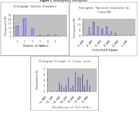
First, the level of homogeneity of SKU data is considered. This step has a twofold objective. First to give a look-and-feel for the data under consideration and, secondly, to provide a benchmark to which other SKU data studies can be compared. Logic suggests that, if SKU data share the same characteristics, then the use of a single forecasting method tailored to these would be justified (as in the case of Robust Trend for the Telecommunications data, Fildes et al. (1998)).

Three homogeneity metrics as proposed in Fildes et al. (1998) have been considered here. Firstly, the differences zt=(xt-xt-1) are computed, where the observed time series

is x1 ,...,xn . Since outliers distort measures of trend and variation, they should be

identified and removed (Nikolopoulos and Assimakopoulos 2003, Adya et al. 2001). If the upper and lower quartiles of zt are Uz and Lz respectively, an observation is

defined as an outlier if:

zt < Lz – 1.5(Uz -Lz) or, if zt > Uz + 1.5(Uz -Lz)

Any outliers are removed from the series zt and replaced with the boundary values Lz – 1.5(Uz - Lz) and Uz + 1.5(Uz -Lz) respectively. This procedures run only once,

resulting in a modified series xt/, although it could potential generate meta-outliers

(Nikolopoulos 2003); in other words the removal of an outlier could generate a huge first difference resulting in new outliers in neighbouring positions.

The strength of the linear trend can be measured by the correlation between xt’ and t,

the higher the absolute value of the correlation, the stronger the linear trend. The level of randomness can be measured by regressing xt/on t, xt-1/, xt-2/ and xt-3/ (this general

linear-autoregressive model approximates the systematic variation in timeseries). The corrected R2 measures the variation explained by the autoregressive model. Histograms of these measures can help identify the characteristics of a data set (Fildes

[Insert Figure 1 about here]

Figure 1 shows the “best” behaved FMPs series for this company (44 in total), that is data series with at least 24 months of non-zero sales history. It is observed that the company data present on average one outlier, medium-to-strong linear positive trend and medium-to-large random component. This contrasts with the M-data or the telecommunications data series characteristics (Fildes et al. 1998). The M-data have been seen to exhibit strong positive trend, medium variation about the trend and some outliers, while the telecommunications data have been seen to exhibit negative trend, low variation about the trend and several outliers.

4. Evaluation

The company is mainly focussed on one-month ahead forecasts as well as a total annual forecast. The forecasting team consists of a forecasting manager and two other supporting staff. The company forecasting process consists of the following steps:

• Adjustments to original data are imposed due to historical irregular events

• An exponential smoothing method based FSS is used for the production of baseline forecasts

• Judgmental interventions are applied

• Notes for every adjustment are made

• No evaluation of the impact of the judgmental adjustments is made

Forecasts of the 44 SKUs under consideration for a period of 3 months were available, yielding 132 triplets (actual sales, system forecast and final forecast). In these 132 cases, 71 included judgmental adjustments where the final forecast was different than the system forecast amounting to 54% of the cases.

The major issue from the literature is whether the judgemental adjustment process lead to improved accuracy. Although the various Diamantopoulos/ Mathews papers are supportive and Sanders and Ritzman (2001) provide a summary of when adjustments are thought to be most worthwhile, Armstrong and Collopy (1998) is much more sceptical, doubting their value in most circumstances including those where company experts as here are involved. In addition to providing much more complete evidence than has been previously examined, we seek to understand the types of adjustment that have been made and where errors are introduced. The aim is to offer guidance as to the circumstances when adjustment is most effective. We therefore examine:

• Direction: how often do the forecasters adjust in the wrong direction?

• Size: does the forecaster tend to make adjustments which undershoot or overshoot?

• Attitude to information: is there any tendency to adjust in particular directions or is positive information (with a correspondingly positive adjustment) as likely to improve accuracy as information with a perceived negative impact. In addition, is positive information weighted similarly to negative?

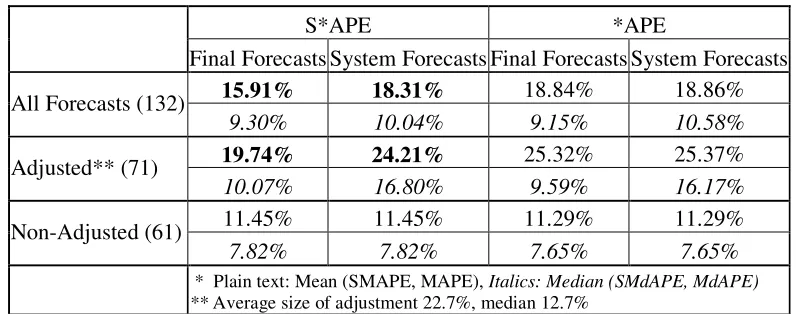
[Insert Table 1 about here]

Starting by examining Table 1, using SMAPE as the metric, a clear gain from the judgmental interventions can be identified. This is due to some huge errors resulting from very small actual values that consequently affect the MAPE metric. Thus, the overall accuracy for the 71 adjusted cases, drops from 24.3 % down to 19.7%, an improvement of almost 5 points! If we translate that gain to the total set of 132 forecast triplets, the overall gain is from 18.3 % down to 15.9%

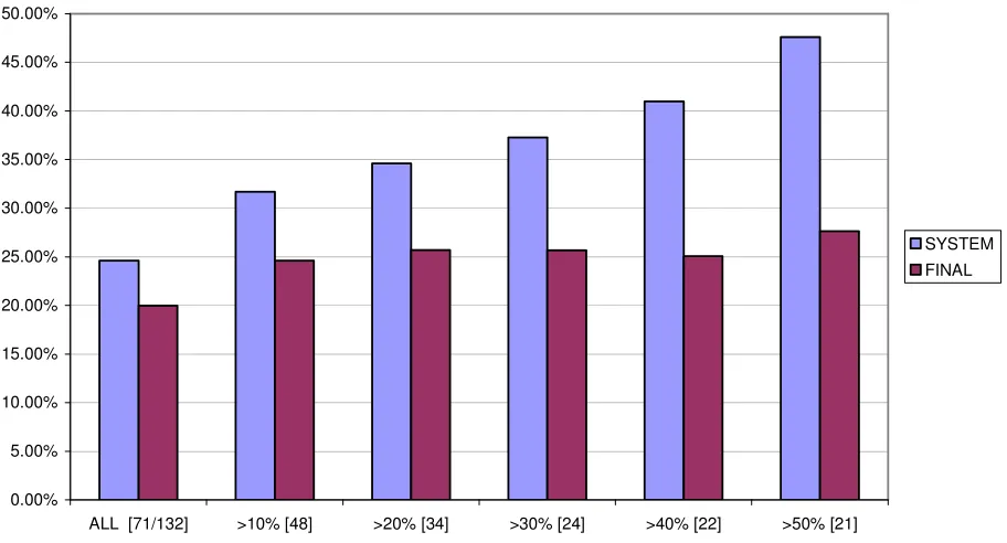
[Insert Figure 2 about here]

accuracy gain of the final vs. the system forecast, resulting from the imposed adjustments. The next bar shows the gain from adjustments over 10%, over 20%, etc. It is obvious that the forecasting accuracy gain comes from the major adjustments, those greater than 10% or even 20%. The last bar representing adjustments over 50% (21 cases) results in an accuracy gain of almost 20% (SMAPE)! So, the more the adjustment, the more the gain. This indicates that when major adjustments are made, they result in major accuracy advances. There is some evidence from the FSS where ‘notes’ are recorded that these occur when the forecaster has specific knowledge over a forthcoming irregular event (i.e. a promotion),

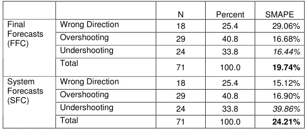
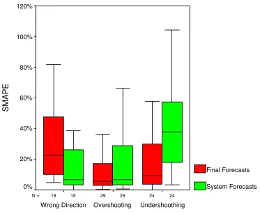
Of the types of mistakes a forecaster can make, how often does the forecaster adjust in the wrong direction? Do they tend to undershoot or overshoot? Grouping the 71 adjustments into three categories based on the direction and size of the forecast errors (table 2):

• In 25% of the cases the adjustment is in wrong direction!

• In 41% of the cases the adjustment is in correct direction but leads to

overshooting theactual

• In 34% of the cases the adjustment is in correct direction but is too little (an

undershoot).

Hence, there is no dominant type of error being made. But given that the cause for adjustment is generally to reflect a promotion, it probably should be a cause for concern that 25% of the adjustments are in the wrong direction.

[Insert Table 2 about here]

[Insert Figure 3 about here]

Figure 3 clearly illustrates this conclusion, showing that all the gain comes only from the case of adjusting the forecast in the right direction but on the condition that the forecaster does not overshoot.

[Insert Figure 4 about here]

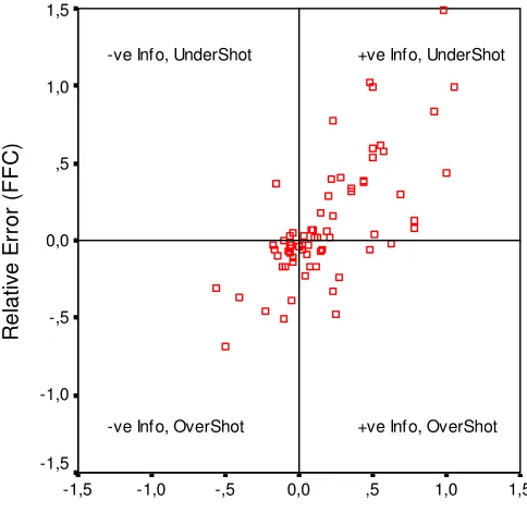
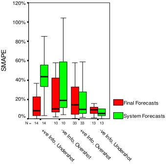
The attitude of the forecaster in interpreting the intelligence - the additional information, resulting in positive or negative adjustments respectively, is presented in Figure 4. In this figure we graph the Relative Adjustment (adjustment divided by the system forecast), versus the Relative Error (final forecast error divided by the system forecast). Positive Adjustment is driven from positive information and vice versa. Positive Error results from Undershooting (Err>0=>Act-FFC>0=>FFC<Act) and vice versa. The majority of cases lie in the first and third quarters. Positive information leads to major undershooting while negative information to conservative overshooting. In this graph we have excluded one extreme case where the Relative adjustment was more than 300%, that is the adjustment was more than three times the system forecast. So based on the remaining 70 cases, viewing forecasting accuracy through the Attitude to Information perspective we end up with table 3.

[Insert Table 3 about here]

[Insert Figure 5 about here]

In the Box-plot in figure 5 this becomes even clearer where the majority of the accuracy gain comes from this small number of positive but conservative adjustments.

5. Discussion

So far straightforward comparison of final and system forecasts shows a major improvement in accuracy; however, are these adjustments optimal? One way to examine this hypothesis is by running the following regression:

SFC SFC FFC b a SFC

SFC

ACT− _{= +} −

(1)

where, ACT: Actual sales, FFC: Final Forecasts, SFC: System Forecasts, or:

RelERR = a +b RelADJ (2)

where, RelERR: Relative error, RelADJ: Relative adjustment

If a=0 and b=1 then (ACT = FFC + error), thus the adjustment is optimal! If a 0 then there is systematic error term (a*SFC) that disturbs optimality while If b 1 the forecaster systematically over or under adjusts. Calculating this regression gives the following results:

RelERR = .404 RelADJ [71 cases, Sig=.000]

The constant term was not found statistically different to zero in this model, so it was omitted and the second coefficient b was recalculated. The residuals are well-behaved and there is no evidence of heteroskedasticity in this model, and other aspects of the residuals are well behaved. In this case where a=0, formula (2) with some trivial algebraic manipulations can be rewritten as:

where, ADJ: Adjustment= FFC-SFC, so it is more clear this way that:

• If b=1 => ACT = SFC + ADJ = FFC => Ideal Adjustment

• If b<1 => ACT = SFC + b ADJ < FFC => Overshoooting

• If b>1 => ACT = SFC + b ADJ > FFC => Undershoooting

Thus, the previous result can be rewritten as:

ACT = SFC + .404 ADJ, [71 cases, Sig=.000]

The coefficient .404 is positive as expected, however significantly less than unity. It is obvious that the adjustment is too high in many cases. Examining the same regression from the adjustment direction perspective we end up with the following formulas1:

Wrong direction ACT = SFC - .457 ADJ [18 cases, Sig=.017]

Overshooting ACT = SFC + .232 ADJ [29 cases, Sig=.001]

Undershooting ACT = SFC + 1.492 ADJ [24 cases, Sig=.000]

As expected2 in the case of adjusting in the wrong direction a negative coefficient is calculated. Furthermore, when overshooting the coefficient is substantially less than unity (a case of serious over adjusting), while when undershooting the coefficient is greater than unity. Thus, the forecasting gain comes in practice from this third type of adjustment.

1 _{Constant term a statistically equals to 0, therefore drops in all three cases.}

Re-calculating these formulas respectively to the attitude of the forecaster to the additional information provides very interesting results:

Positive Information ACT = SFC + .379 ADJ [48 cases, Sig=.000]

Negative Information ACT = SFC + .900 ADJ [23 cases, Sig=.001]

So when adjusting with negative information the forecasters are much closer to the ideal case of rational adjustment (with b=1).

6. Conclusions

The current study has examined the benefits of judgmental interventions on SKUs forecasts by comparing the actual sales both to system and final forecasts. The findings support the case that adjustments improve accuracy significantly, especially when they are:

• of a substantial size (over 10%) usually backed up by domain knowledge

• in the right direction but do not overshoot! (Particularly for positive adjustments.)

As far as perspective is concerned, this study in a way is like setting free “Aeolus’ imprisoned storm-Winds”. This exaggeration tries to indicate the inattention shown, historically to SKUs, although these data play an important role in manufacturing and retailing activities.

Unavoidably, many research issues have been raised and need further research - some of these will be addressed in future studies during this project, including

• A longitudinal extension of the current study: the results presented here are base on thee consecutive periods. It is important to establish the robustness of these results over time

• An analysis designed to compare system forecasts with those derived from classical extrapolation techniques, as well as established FSSs: this is an essential study in order to assess the potential gains that could be obtained from the adoption of more advanced FSSs.

• Rationality analysis: are the provided forecasts unbiased and efficient? Are forecasts updates consistent? This can only be addressed when more forecast sets are available per SKU series.

• The determinants of the forecasts: last but not least, what are the dominant drivers of the final forecast, the system forecasts or judgment?

Acknowledgements

References

Adya, M., Collopy F., Armstrong, J. S. & Kennedy, M., (2001). Automatic identification of time series features for rule-based forecasting. International Journal of Forecasting 17, 143-157.

Armstrong, J.S. and Collopy, F. (1998), "Integration of statistical methods and judgment for time series forecasting: principles from empirical research", In Wright, G and Goodwin, P (Eds) Forecasting with Judgment, Chichester: Wiley. Balkin, S. and Ord, K. (2000). Automatic neural net modelling for univariate time

series, International Journal of Forecasting 16, 509-515.

Chatfield, C. (1993). A personal view of the M2-Competition, International Journal of Forecasting 9, 23-24.

Fildes, R., Goodwin, P. & Lawrence, M. (2005). Design features of Forecasting Support Systems and their effectiveness, Decision Support Systems, forthcoming.

Fildes, R., Hibon, M., Makridakis, S., & Meade, N. (1998). Generalising about univariate forecasting methods: further empirical evidence. International Journal of Forecasting 14, 339-358.

Fildes, R. & Beard, C. (1992). Forecasting systems for production and inventory control, International Journal of Operations and Production Management 12, 4-27.

Gardner, E. S. Jr. & Anderson E. A. (1997) Focus forecasting reconsidered,

International Journal of Forecasting 13, 501-508.

Gardner, E. S. Jr. & McKenzie, E. (1985), Forecasting trends in time series,

Management Science 31, 1237-1246.

Goodwin, P. (2000). Improving the voluntary integration of statistical forecasts and judgment. International Journal of Forecasting 16, 85-99.

Goodwin, P. (2002). Integrating management judgment with statistical methods to improve short-term forecasts. Omega: International Journal of Management Science 30, 127-135.

Goodwin, P. & Lawton, R. (1999). On the asymmetry of the symmetric MAPE..

International Journal of Forecasting 15, 405-408.

Goodwin, P. & Wright, G. (1994). Heuristics, biases and improvement strategies in judgmental time series forecasting, Omega: International Journal of Management Science 22, 553-568.

Klassen, R.D. & Flores, B.E. (2001). Forecasting practices of Canadian firms: Survey results and comparisons, International Journal of Production Economics 70, 163-174.

Lawrence, M., O'Connor, M. & Edmundson, B. (2000). A field study of sales forecasting accuracy and processes, European Journal Of Operational Research

122, 151-160.

Lawrence, M. & O'Connor, M. (2000). Sales forecasting updates: How good are they in practice?, International Journal Of Forecasting 16, pages 369-382

Lawrence, M.J. (1993). The M2-competition: some personal views. International Journal of Forecasting 9, 25-26.

Lee, H.L., Padmanabhan, V. & Whang, S.J. (1997). Information distortion in a supply chain: The Bullwhip effect, Management Science 43, 546-558.

Makridakis S. & Hibon, M., (2000). The M3-Competition: Results, conclusions and implications, International Journal of Forecasting 16, 451-476.

Makridakis, S., Wheelwright, S. & Hyndman, R., (1998). Forecasting, methods and applications, 3rd _{Edition, Wiley.}

Makridakis, S., Chatfield, C., Hibon, M., Lawrence, M., Mills, T., Ord, K. & Simmons, L. (1993), The M2-Competition - A real-time judgmentally based forecasting study, International Journal of Forecasting 9, 5-22.

Makridakis, S., Andersen, A., Carbone, R., Fildes, R., Hibon, M., Lewandowski, R., Newton, J., Parzen, E. & Winkler, R. (1982). The accuracy of extrapolation (time-series) methods - results of a forecasting competition, Journal Of Forecasting 1, 111-153

Mathews, B.P. & Diamantopoulos, A. (1992). Judgmental revision of sales forecasts - The relative performance of judgementally revised versus nonrevised forecasts,

Journal Of Forecasting 11, 569-576

Mathews, B.P. & Diamantopoulos, A. (1989), Judgemental revision of sales forecasts - A longitudinal extension, Journal of Forecasting 8, 129-140

Mathews, B.P. & Diamantopoulos, A. (1986). Managerial intervention in forecasting: An empirical investigation of forecast manipulation. International Journal of Research in Marketing 3, 3-10.

Mills, T.C. (1993). The M2-Competition: some personal reflections. International Journal of Forecasting 9, 26.

Moon, M.A., Mentzer, J.T. & Smith, C.D. (2002). Conducting a sales forecasting audit. International Journal of Forecasting 19, 133-143

Nikolopoulos, K. and Assimakopoulos, V. (2003), Theta Intelligent Forecasting

Information System, Industrial Management and Data Systems 103, 711-726 Ord, J.K. (1993). Personal views of the M2-Competition. International Journal of

Forecasting 9, 26-28.

Sanders, N and Ritzman, L. P. (2001), "Judgmental adjustment of statistical forecasts", In Armstrong, J.S. (Ed) Principles of Forecasting, Boston: Kluwer.

Tables and Figures

Table 1, Accuracy gain from Judgmental Adjustments

S*APE *APE

_{Final Forecasts System Forecasts Final Forecasts System Forecasts}

15.91% 18.31% 18.84% 18.86%

All Forecasts (132)

9.30% 10.04% 9.15% 10.58%

19.74% 24.21% 25.32% 25.37%

Adjusted** (71)

10.07% 16.80% 9.59% 16.17%

11.45% 11.45% 11.29% 11.29% Non-Adjusted (61)

7.82% 7.82% 7.65% 7.65%

Figure 2, Accuracy gain vs. size of adjustment.

0.00% 5.00% 10.00% 15.00% 20.00% 25.00% 30.00% 35.00% 40.00% 45.00% 50.00%

ALL [71/132] >10% [48] >20% [34] >30% [24] >40% [22] >50% [21]

Table 2, System vs. Final forecasts (SMAPE): Direction and Size of Judgmental Adjustments

N Percent SMAPE

Wrong Direction _{18 25.4 29.06%}

Overshooting _{29 40.8 16.68%}

Undershooting _{24 33.8 16.44%}

Final Forecasts (FFC)

Total 71 100.0 19.74%

Wrong Direction 18 25.4 15.12%

Overshooting 29 40.8 16.90%

Undershooting 24 33.8 39.86%

System Forecasts (SFC)

Figure 3, System vs. Final forecasts (SMAPE): Direction and Size of Judgmental Adjustments

24 29

18 29 24

18 N =

Undershoothing Overshooting

Wrong Direction

S

M

A

P

E

120%

100%

80%

60%

40%

20%

0%

Final Forecasts

Figure 4, Attitude to Information vs. Size of Judgmental Adjustments

Relative Adjustment

1,5 1,0

,5 0,0 -,5

-1,0 -1,5

R

el

at

iv

e

E

rr

or

(

F

F

C

)

1,5

1,0

,5

0,0

-,5

-1,0

-1,5

+ve Info, UnderShot -ve Info, UnderShot

Table 3, System vs. Final forecasts (SMAPE): Attitude to Information and Size of Judgmental Adjustments

Forecasts Attitude to

Information Size of Adjustments N Percent SMAPE

Overshooting _{33 47.1 21.57%}

+ve

Undershooting 14 20.0 12.55%

Overshooting _{10 14.3 21.90%}

-ve

Undershooting 13 18.6 13.44%

Final (FFC)

Total 70 100.0 18.30%

Overshooting 33 47.1 18.33%

+ve

Undershooting 14 20.0 42.98%

Overshooting _{10 14.3 35.49%}

-ve

Undershooting 13 18.6 11.99%

System (SFC)

Figure 5, System vs. Final forecasts (SMAPE): Attitude to Information and Size of Judgmental Adjustments

13 33

10

14 10 33 13

14 N =

-ve _In fo, U

nde rsh_ot +ve

Info_{, O} ver_sho

t -ve _In

fo, O ver_sho

t +ve