s hif t-d e t e c ti o n fo r m o t o r
i m a g e r y-b a s e d b r a i n–c o m p u t e r
i n t e rf a c e
R a z a , H , C e c o t ti, H , Li, Y a n d P r a s a d , G
h t t p :// dx. d oi.o r g / 1 0 . 1 0 0 7 / s 0 0 5 0 0-0 1 5-1 9 3 7-5
T i t l e
Ad a p tiv e le a r n i n g wi t h c ov a r i a t e s h if t-d e t e c ti o n fo r m o t o r
i m a g e r y-b a s e d b r a i n–c o m p u t e r i n t e rf a c e
A u t h o r s
R a z a , H , C e c o t ti, H , Li, Y a n d P r a s a d , G
Typ e
Ar ticl e
U RL
T hi s v e r si o n is a v ail a bl e a t :
h t t p :// u sir. s alfo r d . a c . u k /i d/ e p ri n t/ 3 7 7 0 7 /
P u b l i s h e d D a t e
2 0 1 6
U S IR is a d i gi t al c oll e c ti o n of t h e r e s e a r c h o u t p u t of t h e U n iv e r si ty of S alfo r d .
W h e r e c o p y ri g h t p e r m i t s , f ull t e x t m a t e r i al h el d i n t h e r e p o si t o r y is m a d e
f r e ely a v ail a bl e o nli n e a n d c a n b e r e a d , d o w nl o a d e d a n d c o pi e d fo r n o
n-c o m m e r n-ci al p r iv a t e s t u d y o r r e s e a r n-c h p u r p o s e s . Pl e a s e n-c h e n-c k t h e m a n u s n-c ri p t
fo r a n y f u r t h e r c o p y ri g h t r e s t r i c ti o n s .
1
Haider Raza*, Hubert Cecotti*, Yuhua Li†, and Girijesh Prasad*
2
*Intelligent Systems Research Centre, School of Computing and Intelligent Systems, Ulster University, 3
Londonderry, UK. 4
†School of Computing, Science and Engineering, University of Salford, Manchester, UK. 5
[email protected], [email protected],[email protected] , [email protected]
6 7
Abstract—A common assumption in traditional supervised learning is the similar probability distribution of 8
data between the training phase and the testing/operating phase. When transitioning from the training to 9
testing phase, a shift in the probability distribution of input data is known as a covariate shift. Covariate shifts 10
commonly arise in a wide range of real-world systems such as, electroencephalogram (EEG) based brain-11
computer interfaces (BCIs). In such systems, there is a necessity for continuous monitoring of the process 12
behavior, and tracking the state of the covariate shifts to decide about initiating adaptation in a timely 13
manner. This paper presents a covariate shift-detection and -adaptation methodology, and its application to 14
motor imagery based BCIs. A covariate shift-detection test based on an exponential weighted moving average 15
(EWMA) model is used to detect the covariate shift in the features extracted from motor imagery based brain 16
responses. Following the covariate shift-detection test, the methodology initiates an adaptation by updating the 17
classifier during the testing/operating phase. The usefulness of the proposed method is evaluated by using real-18
world BCI datasets (i.e. BCI Competition IV dataset 2A and 2B). The results show a statistically significant 19
improvement in the classification accuracy of the BCI system over traditional learning and semi-supervised 20
learning methods. 21
22
Keywords— Adaptive learning, brain-computer interfaces, covariate shift-detection, transductive learning.
23
I.
I
NTRODUCTION24
25
In traditional machine learning techniques, data are assumed to be drawn from stationary distributions. While
26
training a traditional supervised classifier, it is commonly assumed that the input data distribution in the training set
27
and the testing set follows the same probability distribution (Bishop 2006; Duda et al. 2001; Grossberg 1988; Kelly
28
et al. 1999; Mitchell 1997; Vapnik 1999). However, in real-world applications, processes are non-stationary, and are
29
often characterized by a shifting nature, as the data distribution may shift over time. With applications working in
30
non-stationary environments (NSEs), the data distribution shifts over time; in general this may be due to thermal
31
drift, ageing effects, and noise. The scenario where the training set and testing set follow different distributions but
32
the conditional distribution remains unchanged is known as covariate shift (Sugiyama et al. 2007; Li et al. 2010). In
33
most of the real-world applications, non-stationarity is quite common, especially with the systems interacting with
34
the dynamic and evolving environments, e.g., data coming from electroencephalogram (EEG) based brain-computer
35
interfaces (BCIs), share price prediction in stock market, and wireless sensor networks. Achieving high classification
36
accuracy in a BCI is a particularly challenging task because the signals may be highly variable over time.
37
Adaptive Learning with Covariate
Shift-Detection for Motor Imagery based
1
A BCI is an alternative communication’s means, which allows a user to express his or her will without muscle
2
exertion, provided that the brain signals are properly translated into computer commands (Wolpaw et al. 2002). With
3
an EEG based BCI that operates online in real-time non-stationary/changing environments, it is required to consider
4
input features that are invariant to shifts of the data during long and across sessions, or learning approaches that are
5
able to detect the changes that may repeat overtime, to update the classifier in a timely fashion. The non-stationarities
6
in the EEG may be caused by various reasons such as changing user attention level, electrode placement, and user
7
fatigue (Li et al. 2010; Blankertz & Tomioka 2008; Arvaneh, Cuntai, et al. 2013; Raza et al. 2015). Due to these
non-8
stationarities, it is expected to find notable variations or shifts in the EEG signals during trial-to-trial, and
session-to-9
session transfers (Li et al. 2010; Raza et al. 2013a; Blankertz et al. 2002; Raza et al. 2015; Arvaneh, Guan, Ang, et al.
10
2013). These variations often appear as covariate shifts in the EEG signals, wherein the input data distributions differ
11
significantly between training/calibration and testing/operating phases, while the conditional distribution remains the
12
same (Raza et al. 2013b; Satti et al. 2010; Sugiyama 2007; Shimodaira 2000; Raza et al. 2014). To date, the low
13
classification accuracy has been one of the main concerns of the developed BCI systems based on a motor imagery
14
(MI) detection, which directly affects the reliability of the BCI (Li et al. 2010; Blankertz & Tomioka 2008; Rezaei et
15
al. 2006). To enhance the performance of BCI systems, several feature extraction, feature selection, and feature
16
classification techniques have been proposed in the literature (Shahid & Prasad 2011; Suk & Lee 2013; Kuncheva &
17
Faithfull 2014; Buttfield et al. 2006; Vidaurre et al. 2006; Coyle et al. 2009; Ramoser et al. 2000; Arvaneh, Cuntai, et
18
al. 2013; Arvaneh, Guan, et al. 2013). A large variety of features have been used in MI based BCI such as band
19
powers, power spectral density, time frequency features, and common special patterns (CSP) based features.
20
However, due to brain’s non-stationary characteristics, the spatial distribution of the brain evoked responses may
21
change over time, resulting in shifts in feature distributions.
22
23
The main drawback of the solutions proposed in the related literature is the requirement of labeled data before
24
starting the adaptation in the evaluation/operating phase (Li et al. 2010; Sugiyama 2012). Additionally, most of the
25
shift-detection methods present in the literature are based on the batch processing for a dataset shift detection (Gama
26
et al. 2013; Alippi et al. 2013; Elwell & Polikar 2011), so there is a time delay in shift-detection. Hence, for real-time
27
systems, the batch processing methods are not beneficial where initiating adaptation in the nick-of-time is of supreme
28
interest. In this paper, we present a novel design methodology for an adaptive classification, which monitors the
29
covariate shift in the input streaming data (i.e., EEG features) through an exponential weighted moving average
30
(EWMA) model based covariate shift-detection (CSD) test (Raza et al. 2013a; Raza et al. 2013b). The CSD test
31
operates in two stages, the first stage deals with covariate shift-detection, and the second stage corresponds to the
32
covariate shift validation. This two stage structure helps in reducing the false detection rate, which may reduce an
33
unnecessary retraining of the classifier. The classifier adaptation is only initiated once the covariate shift is confirmed
34
using validation; after validation, the classifier is retrained based on the updated knowledge base (KB) discussed later
35
in Section IV. The proposed method uses different adaptation mechanisms to update the knowledge base (KB i.e.,
training data) of the classifier on the new knowledge. In the first method, a transductive learning approach is used to
1
add the relevant information in to the KB after each CSD. Moreover, the transductive learning is only used to
2
increase the size of KB, but the overall classification is performed using an inductive classifier. In second method,
3
the KB is updated incrementally using the correctly predicted labels after each CSD. The experiments on the
real-4
world datasets are used to show that the covariate shift can be adapted using the proposed method. Using the data
5
from the BCI competition-IV 2A and -2B, we have demonstrated that the proposed method can outperform a
6
traditional learning approach and other competing methods. The novel contributions for the paper can thus be
7
summarized as follows:
8
9
A covariate shift-adaptation model is introduced to address the effects of non-stationarity in the EEG signals.
10
An EWMA based CSD test is applied to detect the non-stationary changes in the principal component analysis
11
(PCA) based features of the motor imagery based brain responses.
12
Third, the proposed model updates its classification decision boundary online without making any a-priori
13
assumption about the distribution for the upcoming test data.
14
15
In this paper, we extend the study of adaptive learning with covariate shift-detection (Raza et al. 2014) by
16
conducting an extensive experimental evaluation on motor imagery based BCI datasets. In particular, our main
17
focus is to account for covariate shift which may arise during session-to-session transfer in BCI experiments. In
18
addition, we perform a thorough analysis on the feature extraction techniques, to extract better discriminative
19
features for the classifier. The remainder of the paper proceeds as follows: First, Section II describes the proposed
20
methodology for the covariate shift-detection, -validation, and -adaptation; Section III presents an application of the
21
method to BCI. Then, the results are detailed in Section IV. Finally, the implications of the results are discussed in
22
Section V.
23
II.
M
ETHODS24
25
A. Problem Formulation
26 27
Let us consider a learning framework in which training dataset is denoted by 𝑋𝑇𝑟= {(𝑥𝑖, 𝑦𝑖)}𝑖=1𝑁 , where 𝑁 is the
28
number of observations, and a target label 𝑦𝑖 is associated with each input 𝑥𝑖. Depending upon the number of inputs 29
and outputs, 𝑥𝑖 and 𝑦𝑖 may be a scalar or vector variables. In the following work, the training dataset is represented 30
as initial knowledge-base (KB). Let us consider a two-class classification problem i.e., 𝑦 ∈ {𝐶1, 𝐶2}., where 𝑦𝑖 = 𝐶1, 31
if 𝑥𝑖 belongs to class 𝜔1, and 𝑦𝑖 = 𝐶2, if 𝑥𝑖 belongs to class 𝜔2. For example, in support vector machine (SVM), we 32
have 𝐶1= −1, and 𝐶2= +1. The probability distribution of the inputs at time 𝑖 can thus be defined as, 𝑃(𝑥𝑖) = 33
𝑃(𝜔1)𝑃(𝑥𝑖|𝜔1) + 𝑃(𝜔2)𝑃(𝑥𝑖|𝜔2) where 𝑃(𝜔1) , 𝑃(𝜔2) are the prior probabilities of getting a sample of the classes 34
The goal is to predict the labels of upcoming samples (𝑦̂)𝑖 resulting into 𝑋𝑇𝑠 = {(𝑦̂|𝑥𝑖 𝑖)}𝑖=1𝑀 , where 𝑀 is the number 1
of observations in the testing phase.
2
3
B. Algorithm Overview 4
5
The proposed algorithm with the CSD belongs to the category of incremental learning (Elwell & Polikar 2011),
6
where the learning model is updated at each CSD. The covariate shift monitoring is performed using the
CSD-7
EWMA test (Raza et al. 2015; Raza et al. 2013a; Raza et al. 2013b). An advantage of using the CSD test is the
8
enhanced accuracy in terms of low false positives and low false negatives. The proposed algorithm is a single
9
classifier based non-stationary learning (NSL) algorithm that uses the CSD-EWMA test for initiating adaptive
10
corrective action. The algorithm is provided with a time-series training dataset KB, where KB= 𝑋𝑇𝑟, and a 11
classifier ℱ is trained. In the evaluation phase, the CSD-EWMA test is used to monitor and detect the covariate shift.
12
Then, the classifier ℱ is used to classify the upcoming input data 𝑋𝑇𝑠. 13
The key elements of the proposed solution are:
14
15
CSD: CSD test monitors the stationarity of 𝑥𝑖, disregarding their supervised labels. 16
ℱ: The pattern classifier ℱ is used to classify the input samples.
17
KB: The current knowledge base (KB) i.e., updated on each CSD.
18
19
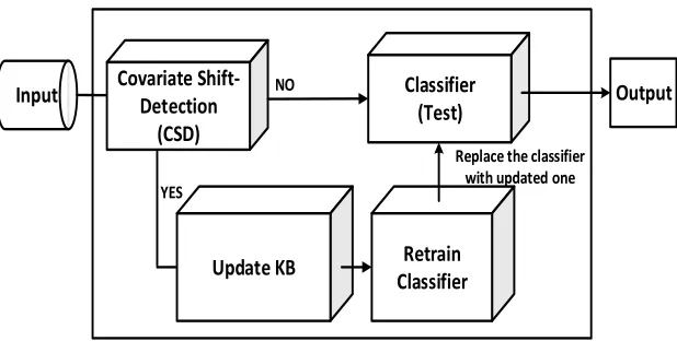
The proposed solution is described in Algorithm 1. After a preliminary configuration phase of the initial classifier
20
ℱ and CSDon KB, the CSD is used to assess the process stationarity. As soon as the CSD-EWMA testdetects a
21
covariate shift in the upcoming unlabeled data, the classifier learned model becomes obsolete, and has to be replaced
22
with a newly configured/retrained model. At each CSD, the new information (i.e., KBNew) becomes available
23
containing the information about the new data distribution. Next, the KBNew is merged with existing KB, and a new
24
KB is prepared. To prepare the updated KB, two methods are identified: first is a transductive learning with CSD
25
(TLCSD), and second is an adaptive learning with CSD (ALCSD). The interactions between the covariate
shift-26
Input Covariate Shift-Detection (CSD)
Retrain Classifier Classifier
(Test) Output
Update KB
Replace the classifier with updated one NO
[image:5.612.159.468.51.207.2]YES
detection, -validation, and -adaptation stages are more clearly illustrated with the help of Fig. 1 and Fig. 2, which are
1
explained in the following subsections.
2
3
Stage-I Shift-Detection (SD-EWMA Test)
Stage-II Shift-Validation
(p-value<0.05)
INPUT
CSD
IF
Yes No
IF
Yes
Shift (No)
Shift (Yes)
No
Classifier
4
Fig. 2: A two-stage covariate shift-detection (CSD). Stage-I is for shift-detection and stage-II works for validation.
5 6
7
Algorithm 1: Learning with CSD
1. Configure the classifier ℱ based on the initial knowledge base KB= 𝑋𝑇𝑟; 2. Configure the parameters λ and L for the CSDtest using the KB;
3. FOR 𝑖 = 1 to length(𝑋𝑇𝑠) 4. Receive new data 𝑥𝑖;
5. IF (CSD detects and validates a non-stationarity at time 𝑖), THEN 6. KB ← KB⋃ KBNew
7. Retrain and adapt the classifier ℱ on KB 8. END
9. Classify the input 𝑥𝑖 by the classifier ℱ and get the predicted label 𝑦̂𝑖 ;
10. END
8
9 10
C. Covariate Shift-Detection (CSD) 11
12
The first step that is required in a CSD test is to detect the covariate shift in the process, possibly without relying
13
on the prior information about the process data distribution before and after the shift. This is a crucial step for
14
reconfiguring the classifier, and it acts as an alarm. The first stage of the test provides an initial estimate of the shift
15
(i.e., where the actual shift has occurred). The first stage test is performed by an SD-EWMA test (Raza et al. 2013a).
16
If the test outcome at the first stage is positive, then the second stage test gets activated, and a validation is performed
17
in order to reduce the number of false alarms (Raza et al. 2013b). The second stage test/validation procedure is
18
discussed in next sub-section. The choice of the smoothing constant λ and a control limit multiplier (L) are the
19
important issue in the EWMA-CSD test. The choice of λ and L are discussed in Section IV.
20
In an EEG-based BCI, the EEG signals are obtained from multiple electrodes, and the application of a feature
1
extraction procedure results in a set of features, hence BCI input data are multivariate. Monitoring of such input
2
processes independently may be misleading, e.g., if the probability that a variable exceeds three-sigma control limits
3
is 0.0027, then a false detection rate of 0.27% is expected. However, the joint probability that 𝑑 variables exceed
4
their control limits simultaneously is (0.0027)𝑑. So, the use of 𝑑-independent control-charts may provide highly
5
distorted outcomes. A principal component analysis (PCA) is therefore used to reduce the dimensionality of the data
6
(Rosenstiel et al. 2012; Kuncheva & Faithfull 2014). It provides fewer components, containing most of the variability
7
in the data. We have used a single component to monitor the shift in the process using SD-EWMA test (Raza et al.
8
2013a) at the first stage.
9
10
D. Covariate Shift-Validation 11
12
According to the Algorithm 1, the KB of the classifier has to be updated at each CSD. However, false positives
13
(i.e., detection that does not correspond to a true shift in the input distribution) result in an unnecessary retraining. To
14
counter this, we have introduced a covariate shift-validation procedure as part of a two-stage structure test (Raza et
15
al. 2013b). This strategy aims at guaranteeing that the classifier relies on an up-to-date KB, and the classifier is only
16
retrained on the occurrence of a valid shift. The covariate shift-validation procedure exploits two sets of observations
17
generated before and at the CSD time point. The observations from the KB are assumed to be in its stationary state,
18
and are compared with data from the current trial, at the CSD time point. To validate the CSD from the stage-I, a
19
multivariate Hotelling's T-Square statistical hypothesis test is used (Hotelling 1947). If the p-value of the test is
20
below 0.05, then the CSD is confirmed, otherwise it is considered as a false-alarm. On each CSD, the KBNew is
21
obtained based on the current shift in the data.
22
23
E. Covariate Shift-Adaptation 24
25
Once the CSD is validated, the adaptation phase starts (see Fig. 2). To adapt to the shift, re-training the classifier
26
is required. In order to retrain the classifier, an additional set of input target pairs is necessary to prepare the KB. To
27
get the set of input target pairs, we have investigated two ways for the KB management. In the first scenario (i.e.,
28
TLCSD), we have applied a transductive-inductive learning model to adapt to a potential covariate shift. However,
29
the transduction part is only used to add new trials into KBNew, and an inductive classifier is used to classify the
30
upcoming samples from the evaluation phase. The transduction part will only start once the covariate shift is detected
31
and validated. In the second scenario (i.e., ALCSD), it is assumed that during the evaluation phase, a true label is
32
available after each trial. Once the covariate shift is detected, then only correctly predicted labels are added into
33
KBNew, the classifier is re-trained, and the updated classifier is used for further classification. This approach is similar
34
to co-training (Zhu 2008) used in a semi-supervised learning (SSL), where the predicted labels are used to train
35
another classifier.
36
Both the methods mentioned above that are used to adapt the classifier in relation to the covariate shift are
1
presented thereafter.
2
3
1) Transductive Learning with CSD (TLCSD) 4
5
A TLCSD model is based on a probabilistic 𝐾-nearest neighbor (KNN) method. Initially, according to Algorithm
6
1, at step 1, an inductive classifier ℱ is trained on the initial KB, and at step 2, the parameters λ and L are set for the
7
CSD test. Once the classifier ℱ is trained, then an evaluation phase starts. At step 3, the parameters λ, L, CRThres, and
8
K are set, wherein CRThres is a confidence ratio threshold that is used to decide the usefulness of the trial, and K is the
9
number of neighbors for the transductive learning. In the evaluation phase, the classifier takes the features as the
10
input obtained from the testing data. The classifier initiates adaptation through transduction after every CSD. Each
11
time the classifier initiates adaptation at step 7, it is considered as one epoch, and it takes ∆m data points to predict
12
the labels through a transductive function 𝒯, where ∆m is the number of points between two shift-detection points,
13
or from the start of evaluation phase to the first detection point. Once the adaptation is initiated at each epoch, the
14
Euclidean distance (𝑑𝑝,𝑞) from the unlabeled data point 𝑥𝑝 to the labeled data point 𝑥𝑞 is computed as given below:
15
16
𝑑(𝑝,q)=‖𝑥𝑝− 𝑥𝑞‖ (1)
17
18
This provides a vector D= [𝑑(𝑝,𝑞1), … , 𝑑(𝑝,𝑞𝑁)] of Euclidean distances from unlabeled data point to the 𝑁 number of
19
labeled data points. Then, the K nearest neighborsare selected. For each of the K nearest points, an RBF kernel is
20
used to compute the weight, as given in equation (2).
21
22
𝐾(𝑝, 𝑞) = 𝑒𝑥𝑝 (−‖𝑥𝑝− 𝑥𝑞‖ 2
2𝜎2 ) (2)
23
From equation (2), we have 0 ≤ 𝐾(𝑝, 𝑞) ≤ 1. A weight with a high value implies the data-point’s closeness to the
24
unlabeled current feature. Thus, the weight for each neighbor is given by:
25
26
𝑅(𝑖) = 𝐾(𝑝, 𝑞𝑖) (3)
27
Using 𝑅(𝑖) and the existing KB, for each of the classes a confidence ratios 𝐶𝑅𝜔i is obtained by,
28
29
𝐶𝑅𝜔1= 𝑃(𝜔1|𝑥) = ∑ 𝑅(𝑖) ∗ (𝑦(𝑖) == 𝜔1) 𝐾
i=1
∑𝐾 𝑅(𝑖)
i=1
(4. 𝑎)
30
𝐶𝑅𝜔2 = 𝑃(𝜔2|𝑥) =
∑𝐾 𝑅(𝑖) ∗ (𝑦(𝑖) == 𝜔2)
i=1
∑𝐾 𝑅(𝑖)
i=1
1
The confidence ratio 𝐶𝑅𝜔𝑖attained from equation (4.a & 4.b) may be viewed as a posterior probability of the class
2
membership of the current unlabeled data point, as 𝐶𝑅𝜔1+ 𝐶𝑅𝜔2= 1. This 𝐶𝑅𝜔𝑖acts as a belief or confidence,
3
which determines if a data sample belongs to a particular class. In this step, for each observation from the ∆𝑚 data
4
points are obtained, and 𝐶𝑅𝜔𝑖 to decide if both the trial’s features and the estimated output labels should be added to
5
the existing knowledge-base i.e. if max (𝐶𝑅𝜔1, 𝐶𝑅𝜔2) > CRThres, then the couple (EEG signal corresponding to the
6
trial, estimated output label) is added into KBNew, otherwise it is discarded. At step 7, this KBNew is then merged into
7
the existing KB. Based on the updated KB, the inductive classifier function is updated, and a new classifier ℱ is
8
obtained at step 8. Every time a new KBNew is created, the classifier ℱ is updated, and this process is repeated until all
9
the M points in the testing phase are classified.
10
11
2) Adaptive Learning with CSD (ALCSD)
12 13
In ALCSD, initially at step 1 of Algorithm 1, an inductive classifier ℱ is trained with the initial KB of 𝑁 labeled
14
trials. Using KBat step 2, the parameter λ is obtained for the CSD test, and the control limit (L) for the CSD is set to
15
L=2. Then, an evaluation phase starts at step 4, and unlabeled features from 𝑋𝑇𝑠 are processed sequentially for 16
classification. At step 6, the CSD test is used to monitor the covariate shift. Once the covariate-shift is detected, it
17
acts as an alarm to update the classifier. To update the classifier, new knowledge from the data is required. In order to
18
obtain KBNew, it is assumed that in each trial, the true label is available, and among all predicted labels only correctly
19
predicted labels through an inductive classifier are added into KBNew. KBis updated with the content of KBNew at step
20
7. KB is used to retrain the classifier at step 8, and further at step 10, this updated classifier is used to classify the
21
upcoming data. On each CSD, KB gets updated, and a new classifier is created.
22
23
III.
A
PPLICATION TOB
RAIN-C
OMPUTERI
NTERFACE 241) Data Description
25
26
a) BCI Competition IV dataset 2A 27
28
The BCI Competition IV dataset 2A (Tangermann et al. 2012) is comprised of the EEG data collected from nine
29
subjects, namely [A01-A09], that were recorded during two sessions on separate days for each subject. The data
30
consists of 25 channels, which include 22 EEG channels, and 3 monopolar EOG channels. Among the 22 EEG
31
channels, 10 channels are selected for this study, which are responsible for capturing most of the motor imagery
32
activities. The selected channels are presented in Fig. 3(a). The data was collected on four different motor imagery
33
tasks: left hand (class 1), right hand (class 2), both feet (class 3), and tongue (class 4). Each session consists of six
34
runs separated by short breaks, each run comprised of 48 trials (12 for each class). The total numbers of 288 trials are
35
in each session. Only the class 1 and the class 2 for left hand and right hand were considered in this study (i.e., 144
trials). For more details about the dataset kindly refer (Tangermann et al. 2012). The motor imagery data from the
1
session-I was used to train the classifiers, and the motor imagery data from the session-II was used as the test dataset.
2
3
b) BCI Competition IV dataset 2B 4
5
BCI competition 2008-Graz dataset B (Tangermann et al. 2012) is a dataset consisting of EEG data from 9
6
subjects, namely [B01-B09]. Three channel bipolar recordings (C3, Cz and C4) were acquired with a sampling
7
frequency of 250 Hz, the montage is depicted in Fig. 3(b). All signals were recorded monopolarly with the left
8
mastoid serving as reference, and the right mastoid as ground. For each subject, five sessions are provided. The
9
motor imagery data from session-I & -II were used to train the classifiers, the data from session-III was used to
10
obtain the hyperparameters (i.e., K and CRThres), and the motor imagery data from session-IV & -V were used to
11
evaluate the performance of the test. Session-IV & -V consist of 160 trials each. Each trial is a complete paradigm of
12
8 seconds, for more details refer to (Tangermann et al. 2012).
13
14
2) Data Processing and Feature Extraction 15
16
a) Temporal Filtering 17
18
C3
Ref Gnd
C1 C5
CP3 FC3
C4 C6 C2
CP4 FC4
Ref Gnd
C3 Cz C4
[image:10.612.207.453.51.188.2](a) (b)
Fig. 3. Electrode montage corresponding to the international 10-20 system: (a) Dataset 2A, among all 22 EEG channels, total 10 channels are selected as shown in black filled hollow circles. (b) Dataset 2B, all channels are selected.
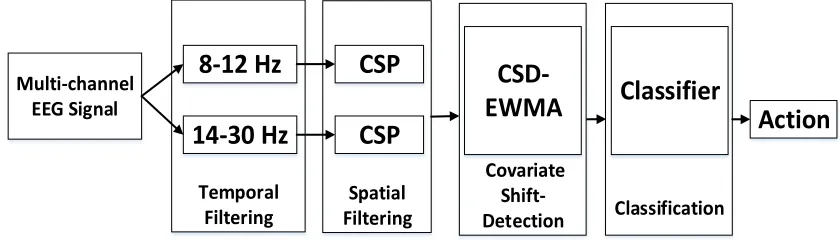
Spatial Filtering Multi-channel
EEG Signal
Temporal
Filtering Classification
8-12 Hz
14-30 Hz
CSP
Classifier
CSP
Action
Covariate Shift-Detection
CSD-EWMA
Fig.4: Block diagram for the MI based BCI. It consist of following five stages: Initially the multichannel EEG signals are acquired, next the band-pass filtering is performed, and then the CSP features are obtained, and the covariate shift is monitored, and then features are classified
[image:10.612.101.521.230.350.2]The second stage of the MI based BCI block diagram (see Fig. 4) employs two filters that decompose the EEG
1
signals into two different frequency bands. Two band-pass filters are used, namely [8-12] Hz (µ band) and [14-30]
2
Hz (β band). These frequency ranges are used because they cover a stable frequency response related to MI
3
associated phenomena of event-related synchronization and de-synchronization (ERS/ERD). In the next sections, we
4
consider a time segment of 3 s after the cue onsets for both data sets. 5
6
b) Spatial Filtering 7
8
The third stage employs a spatial filter that maximizes the variance of spatially filtered signals under one
9
condition, while minimizing it for the other condition. Raw EEG scalp potentials are known to have poor spatial
10
resolution due to volume conduction. If the signal of interest is weak while other sources produce strong signals in
11
the same frequency range, then it is difficult to classify two classes of EEG measurements (Blankertz et al. 2008).
12
The neurophysiological background of motor-imagery based BCIs is that motor activity, both actual and imagined,
13
causes an attenuation or increase of localized neural rhythmic activity called Event-Related Desynchronization
14
(ERD) or Event-Related Synchronization (ERS). The Common-Spatial-Pattern (CSP) algorithm is highly successful
15
in calculating spatial filters for detecting (ERD/ERS) (Ang et al. 2012; Ang et al. 2008). The objective of the CSP
16
algorithm is to compute features whose variances are optimal for discriminating two classes of brain evoked
17
responses in EEG signal.
18
19
A pair of band-pass and spatial filters in the first and second stages perform spatial filtering of EEG signals that
20
have been band-pass filtered in a specific frequency range. Thus, each pair of band-pass and spatial filter computes
21
the CSP features that are specific to the band-pass frequency range. CSP is a technique to analyze multichannel data
22
based on the recording from two classes (Blankertz et al. 2008). It is a data driven supervised decomposition of
23
signals parameterized by a matrix 𝑾 ∈ ℝ𝐶×𝐶 (C: number of selected channels) that projects the single trial EEG
24
signal 𝑬 ∈ ℝ𝐶 in the original sensor space to 𝐙 ∈ ℝ𝐶, which lives in the surrogate sensor space, as follows:
25
26
𝐙 = 𝑾𝑬 (5) 27
28 29
where 𝑬 ∈ ℝ𝐶×𝑇 is a EEG measurement data of single trial, C is the number of channels; T is the number of
30
samples per channel. W is the CSP projection matrix. The rows of W are the spatial filters, and the columns of W are
31
the common spatial patterns. The spatial filtered signal Z given in eq. (5) maximizes the difference in the variance of
32
the two classes of EEG measurements. A CSP analysis is applied in order to obtain an effective discrimination of
33
mental states that are characterized by ERD/ERS effects. However, the variances of only a small number (m) of the
34
spatial filtered signal are generally used as feature for classification. The 𝑚 first and last rows of Z i.e. 𝒁𝒕, t∈ 35
{1 … 2𝑚} form the feature vector 𝒙𝒕given by: 36
𝒙𝒕= 𝒍𝒐𝒈 ( 𝒗𝒂𝒓(𝒁𝒕)
∑𝟐𝒎𝒊=𝟏𝒗𝒂𝒓(𝒁𝒊)) (6)
1
2 3
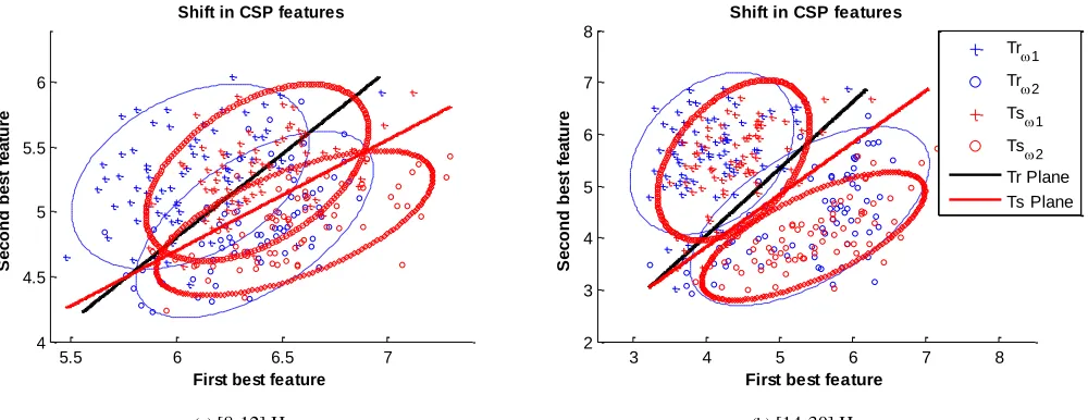
Here, m=1. The CSP features from both frequency bands are combined to form the input features for training a
4
classifier. Fig. 5 shows the covariate shift in the CSP features for both training and test datasets for subject A03 over
5
two different frequency bands mu (µ) [8-12] Hz and beta (β) [14-30] Hz. The blue crosses and red circles denote the
6
features of the left hand and right hand motor imagery, respectively. The black line and red line represent the
7
separation planes between the features of two classes obtained from two frequency bands as training and testing
8
features, respectively. The separation planes are plotted for illustration purpose only.
9
10
3) Covariate Shift-Detection (CSD) 11
12
The fourth stage uses the CSD test on the CSP features. In both datasets, the data are generated from multiple
13
channels, and for each channel two features are produced from each frequency band. To use CSD-EMWA, PCA is
14
used to reduce the number of the features, and a single component is used to detect the covariate shift. To execute the
15
CSD test, the smoothing constant λ is selected for each subject based on minimizing the sum of squares of
1-step-16
ahead prediction error method, and the control limit multiplier is set to L=2. The choice of L has a major impact on
17
the performance of the CSD test, a small value of L makes it more sensitive in detecting minor shifts in the data. The
18
CSD test in the operational stage detects the shifts and validates it through its two stage structure. If the CSD test is
19
positive then a classifier is retrained on the KB.
20
21
[image:12.612.57.557.56.249.2](a) [8-12] Hz (b) [14-30] Hz
Fig. 5: Covariate shift in the EEG dataset 2A-subject A03, between training and testing input distribution for different frequency bands. (a) Mu band [8-12] Hz, and (b) Beta band [14-30] Hz. The red circles denote the features of the left hand motor imagery, and blue crosses denote the features of the right hand motor imagery. The black and red lines represent the decision boundaries obtained by the training data and test data respectively.
5.5 6 6.5 7
4 4.5 5 5.5 6
First best feature
S
e
c
o
n
d
b
e
s
t
fe
a
tu
re
Shift in CSP features
3 4 5 6 7 8
2 3 4 5 6 7 8
First best feature
S
e
c
o
n
d
b
e
s
t
fe
a
tu
re
Shift in CSP features
4) Experimental Setup and Classification Evaluation Metrics
1
2
In order to evaluate the performance of the system, we have considered the classification accuracy (in %) as
3
the measure of index. The experiments are performed using a linear support vector machine (SVM) pattern
4
classifier ℱ. In CSD tests, the percentage (%) of covariate shift-detected and shift-validated are computed as given
5
below:
6
7
% 𝑜𝑓 𝑠ℎ𝑖𝑓𝑡 𝑑𝑒𝑡𝑒𝑐𝑡𝑒𝑑/𝑣𝑎𝑙𝑖𝑑𝑎𝑡𝑒𝑑 = ((#𝑠ℎ𝑖𝑓𝑡 𝑑𝑒𝑡𝑒𝑐𝑡𝑒𝑑/𝑣𝑎𝑙𝑖𝑑𝑎𝑡𝑒𝑑)𝑇𝑜𝑡𝑎𝑙 𝑛𝑢𝑚𝑏𝑒𝑟 𝑜𝑓 𝑡𝑟𝑖𝑎𝑙𝑠 ) × 100 (7)
8
9
The hyperparameters K and CRThres are required to be carefully selected. Two variants of the proposed 10
learning method, namely TLCSD1 and TLCSD2, are therefore presented. In TLCSD1, the hyperparameters are selected 11
based on grid search to maximize the mean accuracy across subjects, with 𝐾 ∈ {6, 12, 18}, and 𝐶𝑅 in the
12
range [0.50 − 1]. In TLCSD2, the hyperparameters are determined for each subject, based on grid search to maximize 13
the accuracy of each subject (subject-dependent). In the dataset 2A, the session-I is divided into two parts, the first
14
80% are used for training the pattern classifier while the remaining 20 % is used to determine the hyperparameters.
15
The evaluation is then performed on the data from session-II. In the dataset 2B, sessions I and II (240 trials) are used
16
for training the pattern classifier, session III (160 trials) is used to obtain the hyperparameters, and sessions IV and V
17
(320 trials) are used to evaluate the performance of the classifier. For each dataset, the accuracy corresponding to a
18
10-fold cross-validation (10-CV) on the training data is provided. Moreover, the two variants for the proposed
19
methods are evaluated and compared with a baseline method and a label propagation based semi-supervised learning
20
(SSL) algorithm. An upper bound (UB) is provided. It is obtained by training the classifier ( ℱ ) on both the training
21
and the test datasets, with an evaluation on the test data. The baseline method uses an inductive learning classifier
22
with CSP features (Ramoser et al. 2000), but it does not adapt/re-train its pattern classifier over time. A graph-based
23
SSL label propagation method (Zhu & Ghahramani 2002) has been considered for comparisons. To compare
24
classifier performance with the baseline method, a two-sided Wilcoxon signed rank test is used to assess the
25
statistical significance of the pairwise comparison at a confidence level of 0.05.
26
27
IV.
R
ESULTS28
29
1) Results for Dataset 2A 30
31
The results corresponding to the choice of the smoothing constant λ and the CSD are presented in Table I. The
32
value of λ is obtained by minimizing the sum of squares of 1-step-ahead prediction errors. In the data of subject A05,
33
a shift was detected 15 times (i.e. 10.42% CSD) whereas it was detected only 7 times for subject A03 (i.e. 4.86%
34
CSD). For subject A05, the CSD decreased from 10.42% to 4.17% after the covariate shift-validation stage, and for
35
subject A03, the CSD decreased from 4.86% to 1.39%. The validation stage thus helps to decrease the rate of false
36
positives at stage-II; consequently the effort of unnecessary retraining the classifier is also reduced.
1
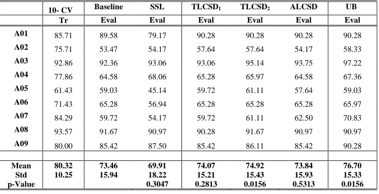
The classification accuracies on dataset 2A, for the different methods and for each subject, are given in Table-II.
2
The 10-CV average classification accuracy on the training dataset is 80.32±10.25%, where subject A08 is having a
3
maximum accuracy of 93.57%. For the baseline results, an inductive classifier is used for the classification on the test
4
data without any adaptation on the CSP features. The baseline method gives an average accuracy of 73.46±15.94%,
5
and subject A03, who has the less number of shifts, has the highest accuracy (92.36%). The SSL label propagation
6
method gives an average accuracy of 69.91±18.22%, which is inferior to the baseline method. In TLCSD1, the
7
parameters K and CRThres have been set to K=18 and CRThres=0.70, and the classification accuracy has improved
8
slightly from 73.46±15.94% to 74.07±15.21%.
9
For TLCSD2, all the subjects have shown an improvement, except for subject A08. The average accuracy of
10
TLCSD2 is 74.92±15.43%, which represents a significant improvement compared to the baseline method (p-value=
11
0.0126). In ALCSD, the results have shown a minor improvement in the performance against the baseline method
12
with the mean accuracy of 73.84±15.93%; only subjects A01, A02, A03, and A07 have shown improvement. The
13
accuracy of UB is 76.70±15.33%, and it represents the performance that can be achieved if all the data are available
14
for training, showing that the knowledge of the test data points in the evaluation of the classifier can improve the
15
TABLEI
RESULTS FOR SHIFT-DETECTION &VALIDATION DATASET 2A.
Subject Lambda
Shift-Detected
Shift-Validated
A01 0.10 11 4
A02 0.80 11 9
A03 1 7 2
A04 1 11 6
A05 0.30 15 6
A06 0.10 14 5
A07 0.10 12 9
A08 0.20 11 5
[image:14.612.117.493.420.613.2]A09 0.50 10 4
TABLE II
CLASSIFICATION ACCURACY (%) RESULTS FROM BCI COMPETITION IV-DATASET 2A
10- CV Baseline SSL TLCSD1 TLCSD2 ALCSD UB
Tr Eval Eval Eval Eval Eval Eval
A01 85.71 89.58 79.17 90.28 90.28 90.28 90.28
A02 75.71 53.47 54.17 57.64 57.64 54.17 58.33
A03 92.86 92.36 93.06 93.06 95.14 93.75 97.22
A04 77.86 64.58 68.06 65.28 65.97 64.58 67.36
A05 61.43 59.03 45.14 59.72 61.11 57.64 59.03
A06 71.43 65.28 56.94 65.28 65.28 65.28 65.97
A07 84.29 59.72 54.17 59.72 61.11 62.50 70.83
A08 93.57 91.67 90.97 90.28 91.67 90.97 90.97
A09 80.00 85.42 87.50 85.42 86.11 85.42 90.28
Mean 80.32 73.46 69.91 74.07 74.92 73.84 76.70
Std 10.25 15.94 18.22 15.21 15.43 15.93 15.33
performance by only 3.23%.
1
2
2) Results for Dataset 2B 3
4
The results for the choice of λ and the CSD are presented in Table III. In this dataset, session IV and V are used for
5
evaluation phase, hence for each session the CSD test is performed independently. In session IV, the subject B01 has
6
the maximum number of CSD (10%), and subject B04 has minimum number of CSD (1.88%). After the covariate
7
shift validation stage, the number of CSD decreased from 10% to 4.38% for subject A01, and the number of CSD
8
decreased from 1.88% to 0.63% for subject A04. Moreover, in session V, subjects B06 and B08 have the maximum
9
number of CSD (10%), and subject B04 has the minimum number of CSD (3.75%). After the covariate
shift-10
validation stage, the number of CSD decreased from 10% to 6.88% for subject B06, and the number of CSD
11
decreased from 10% to 5% for subject B08.
12
13
The classification accuracies on dataset 2B, for the different methods and for each subject, are given in Table-IV.
14
The average accuracy with 10-CV is 70.71±10.78%, with subject B04 obtaining the maximum performance of
15
88.85%. The baseline method gives 65.23±13.98% of average accuracy and subject B04 has the maximum accuracy
16
TABLEIII
RESULTS FOR SHIFT-DETECTION &VALIDATION DATASET 2B.
Subject Lambda Shift-Detected (%)
Shift-Validated (%)
Shift-Detected (%)
Shift-Validated (%)
Session IV Session V
B01 0.10 10.00 4.38 6.88 3.13
B02 0.80 6.88 1.25 9.38 5.63
B03 1 6.88 2.50 8.13 6.25
B04 1 1.88 0.63 3.75 1.25
B05 0.30 7.50 4.38 6.88 3.75
B06 0.10 8.13 5.00 10.00 6.88
B07 0.10 6.25 5.63 7.50 2.50
B08 0.20 6.25 4.38 10.00 5.00
[image:15.612.114.494.532.726.2]B09 0.50 8.13 4.38 8.13 3.75
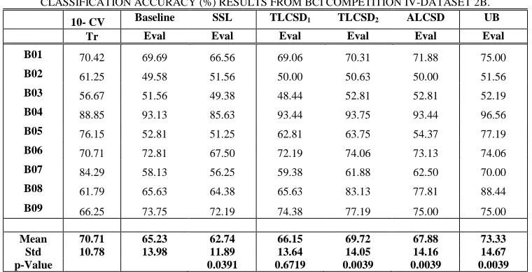
TABLE IV
CLASSIFICATION ACCURACY (%) RESULTS FROM BCI COMPETITION IV-DATASET 2B.
10- CV Baseline SSL TLCSD1 TLCSD2 ALCSD UB
Tr Eval Eval Eval Eval Eval Eval
B01 70.42 69.69 66.56 69.06 70.31 71.88 75.00
B02 61.25 49.58 51.56 50.00 50.63 50.00 51.56
B03 56.67 51.56 49.38 48.44 52.81 52.81 52.19
B04 88.85 93.13 85.63 93.44 93.75 93.44 96.56
B05 76.15 52.81 51.25 62.81 63.75 54.37 77.19
B06 70.71 72.81 67.50 72.19 74.06 73.13 74.06
B07 84.29 58.13 56.25 59.38 61.88 62.50 70.00
B08 61.79 65.63 64.38 65.63 83.13 77.81 88.44
B09 66.25 73.75 72.19 74.38 77.19 75.00 75.00
Mean 70.71 65.23 62.74 66.15 69.72 67.88 73.33
Std 10.78 13.98 11.89 13.64 14.05 14.16 14.67
p-Value 0.0391 0.6719 0.0039 0.0039 0.0039
of 93.13%. The SSL based label propagation method gives 62.74±11.89% average accuracy, which is below the
1
baseline method accuracy. In TLCSD1, the parameters K and CRThres have been fixed to K=18 and CRThres=0.70, and
2
the classification accuracy has slightly improved from 65.23±13.98% to 66.15±13.64%. Next, for TLCSD2, all the
3
subjects have shown an improvement. The average accuracy for TLCSD2 is 69.72±14.05%, being statistically
4
significant better (p-value=0.00039) than the baseline method. In ALCSD, the results have shown a considerable
5
improvement in the performance against the baseline method with the mean accuracy of 67.88±14.16%, which is
6
statistically significant better than the baseline method (p-value=0.0039). Moreover, for ALCSD, all the subjects
7
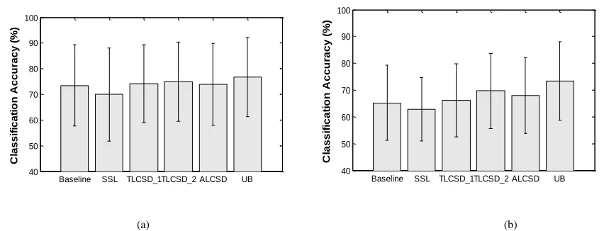
have shown an improvement. The UB method reaches an accuracy of 73.33±14.67%. Fig. 6, presents the average
8
classification accuracy across subjects for both databases (2A and 2B). 9
10
11
12
(a) (b)
[image:16.612.86.512.261.424.2]13
Fig. 6: Comparison of the mean accuracies for the proposed methods against the baseline, SSL, and UB on (a) the dataset 2A and (b) dataset 2B.
14
The represent the standard deviation across subjects.
15
V.
D
ISCUSSION16
The proposed TLCSD and ALCSD methods for the EEG-based BCI are based on a covariate shift-detection and an
17
adaptation framework. An EWMA-CSD test is used to detect the covariate shift. Once the shift is detected, an
18
appropriate adaptive action is initiated to address the effect of the covariate shift. In TLCSD, the new
19
information/knowledge obtained through transduction is used to update the KB (i.e., training data) of the inductive
20
classifier. However, the main classification function is still inductive because the transductive knowledge is only
21
used to add more information into KB.
22
23
An important issue in the CSD is the choice of the control limit multiplier L. Considering small limit L=2 means
24
focusing on minor shifts, such as muscular artifacts arising during trial-to-trial transfer. However, the long term
non-25
stationarities may be accounted for by considering a large value of L=3, such as during session-to-session transfer or
26
run-to-run transfer. We have selected a small value of control limit multiplier L=2, as our aim is to detect the
27
covariate shift that arises during trial-to-trial transfers. The proposed learning techniques make use of CSD to detect
28
the shift and then adapt to non-stationarities in the streaming EEG.
29
Baseline SSL TLCSD_1TLCSD_2 ALCSD UB 40 50 60 70 80 90 100 C la s s if ic a ti o n A c c u ra c y ( % )
1
The parameter CRThres is used to decide whether the information in hand is useful or not. If the information is
2
useful then it is added to the existing KB. The discarded information may come from a different distribution or it
3
may have not provided much confidence to add into KB. The value of CRThres and 𝐾 are important, and are required
4
to be carefully selected in order to achieve superior performance. For instance, for the method TLCSD1, the value of
5
CRThres is empirically selected in the range [0.50-1]. In TLCSD2, the parameters are selected based upon the grid
6
search method and the accuracy is superior for both of the datasets. This implies that the performance of the proposed
7
method mostly depends upon the optimal choice of CRThres.
8
9
The experimental results demonstrated the effectiveness of the proposed covariate shift-detection and adaptation
10
learning strategy. The results showed that the proposed method with CSP filters and optimized parameters is
11
significantly better than the traditional learning methods, and SSL with CSP filters. The combination of EWMA
12
based covariate shift-detection and adaptive learning is thus a good choice for learning in non-stationary
13
environments. The robustness of the CSD test plays an important role in initiating a correct adaptive action.
14
VI.
C
ONCLUSION15
16
The proposed methodology is a flexible tool for adaptive learning in non-stationary environments and effectively
17
accounts for the effect of the covariate shifts. In this paper, two methods (TLCSD and ALCSD) were proposed for
18
the covariate shift-adaptation using a two-stage covariate shift-detection test. The CSD test in the first stage uses the
19
SD-EWMA test; and in the second stage, the multivariate Hotelling's T-Square statistical hypothesis test is used. The
20
CSD test is found very effective in detecting the covariate shifts in the data in real-time. Based on the detected
21
significant shifts, the algorithm initiates adaptive corrective action. The performance of the proposed methods was
22
evaluated on multivariate cognitive task detection problem in the EEG-based BCIs simulated with BCI Competition
23
IV datasets 2A and 2B, and a superior classification accuracy was obtained as both TLCSD and ALCSD have shown
24
statistically significant improvement. This work is planned to be extended further by employing the CSD into the
25
task of fault monitoring.
26
A
CKNOWLEDGEMENT27
H.R. was supported by Ulster University Vice-Chancellor’s research scholarship (VCRS). G.P. and H.C. were
28
supported by the Northern Ireland Functional Brain Mapping Facility project (1303/101154803), funded by
29
InvestNI and the Ulster University. G.P. and H.R. were also supported by the UKIERI DST Thematic Partnership
30
project "A BCI operated hand exoskeleton based neuro-rehabilitation system" (UKIERI-DST-2013-14/126).
31
32
References
Alippi, C., Boracchi, G. & Roveri, M., 2013. Just-In-Time Classifiers for Recurrent Concepts. IEEE Transactions on Neural
1
Networks and Learning Systems, 24(4), pp.620–634. 2
Ang, K.K. et al., 2008. Filter Bank Common Spatial Pattern ( FBCSP ). In Proc. Int’l Joint Conf. Neural Networks (IJCNN). pp. 3
2390–2397. 4
Ang, K.K. et al., 2012. Filter Bank Common Spatial Pattern Algorithm on BCI Competition IV Datasets 2a and 2b. Frontiers in
5
neuroscience, 6, p.39. 6
Ao, J.O. et al., 2014. A Survey on Concept Drift Adaptation. ACM Computing Surveys (CSUR), 4(1), pp.1–44. 7
Arvaneh, M., Guan, C., Ang, K.K., et al., 2013. Optimizing spatial filters by minimizing within-class dissimilarities in 8
electroencephalogram-based brain-computer interface. IEEE Transactions on Neural Networks and Learning Systems, 9
24(4), pp.610–619. 10
Arvaneh, M., Guan, C. & Chai Quek, 2013. EEG Data Space Adaptation to Reduce Intersession Nonstationary in Brain-11
Computer Interface. Journal of Neural Computation, 25, pp.1–26. 12
Bishop, C.M., 2006. Pattern Recognition and Machine Learning, New York: Springer. 13
Blankertz, B. et al., 2008. Optimizing spatial filters for robust EEG single-trial analysis. IEEE Signal Processing Magazine, 14
25(1), pp.41–56. 15
Blankertz, B., Curio, G. & Müller, K.-R., 2002. Classifying single trial EEG: Towards brain computer interfacing. In Advances
16
in Neural Information Processing Systems. pp. 157–164. 17
Buttfield, A., Ferrez, P.W. & Millán, J.D.R., 2006. Towards a robust BCI: Error potentials and online learning. IEEE
18
Transactions on Neural Systems and Rehabilitation Engineering, 14(2), pp.164–168. 19
Coyle, D., Prasad, G. & McGinnity, T.M., 2009. Faster Self-Organizing Fuzzy Neural Network Training and A Hyperparameter 20
Analysis for A Brain-Computer Interface. IEEE transactions on Systems, Man, and Cybernetics., 39(6), pp.1458–71. 21
Duda, R.O., Hart, P.E. & Stork., D.G., 2001. Pattern Recognition, Wiley-Interscience. 22
Elwell, R. & Polikar, R., 2011. Incremental learning of concept drift in nonstationary environments. IEEE Transactions on
23
Neural Networks, 22(10), pp.1517–1531. 24
Grossberg, S., 1988. Nonlinear neural networks: Principles, mechanisms, and architectures. Neural Networks, 1(1), pp.17–61. 25
Hotelling, H., 1947. Multivariate Quality Control-Illsutrated by the Air Testing of Sample Bombsights. Techniques of Statistical
26
Analysis, pp.111–184. 27
Kelly, M., Hand, D. & Adams, N., 1999. The impact of changing populations on classifier performance. In Proceedings of the
28
fifth ACM SIGKDD. ACM, pp. 367–371. 29
Kuncheva, L. & Faithfull, W., 2014. PCA feature extraction for change detection in multidimensional unlabeled data. IEEE
30
Transactions on Neural Networks and Learning Systems, 25(1), pp.69–80. 31
Leeb, R. et al., 2007. Brain-computer communication: motivation, aim, and impact of exploring a virtual apartment. IEEE
32
transactions on neural systems and rehabilitation engineering : a publication of the IEEE Engineering in Medicine and
33
Biology Society, 15(4), pp.473–82. 34
Li, Y. et al., 2010. Application of covariate shift adaptation techniques in brain-computer interfaces. IEEE Transactions on
35
Lotte, F. et al., 2007. A review of classification algorithms for EEG-based brain-computer interfaces. Journal of neural
1
engineering, 4(2), pp.R1–R13. 2
Mitchell, T., 1997. Machine Learning, McGraw Hill. 3
Müller, K.-R. et al., 2004. Machine Learning Techniques for Brain-Computer Interfaces. Machine Learning, 49, pp.11–22. 4
Ramoser, H., Müller-Gerking, J. & Pfurtscheller, G., 2000. Optimal spatial filtering of single trial EEG during imagined hand 5
movement. IEEE Transactions on Rehabilitation Engineering, 8(4), pp.441–446. 6
Raza, H., Prasad, G. & Li, Y., 2014. Adaptive Learning with Covariate Shift- Detection for Non-Stationary Environments. In 7
14th UK Workshop on Computational Intelligence (UKCI), 2014 , IEEE. Bradford, UK, pp. 1–8. 8
Raza, H., Prasad, G. & Li, Y., 2013a. Dataset shift detection in non-stationary environments using EWMA charts. In 9
Proceedings - 2013 IEEE International Conference on Systems, Man, and Cybernetics, SMC 2013. pp. 3151–3156. 10
Raza, H., Prasad, G. & Li, Y., 2013b. EWMA based two-stage dataset shift-detection in non-stationary environments. In IFIP
11
Advances in Information and Communication Technology. Springer Berlin Heidelberg, pp. 625–635. 12
Raza, H., Prasad, G. & Li, Y., 2015. EWMA model based shift-detection methods for detecting covariate shifts in non-stationary 13
environments. Pattern Recognition, 48(3), pp.659–669. 14
Rezaei, S. et al., 2006. Different classification techniques considering brain computer interface applications. Journal of neural
15
engineering, 3(2), pp.139–144. 16
Rosenstiel, W., Bogdan, M. & Sp, M., 2012. Principal component based covariate shift adaption to reduce non-stationarity in a 17
MEG-based brain-computer interface. EURASIP Journal on Advances in Signal Processing, pp.2–8. 18
Satti, A. et al., 2010. A covariate shift minimization method to alleviate non-stationarity effects for an adaptive brain-computer 19
interface. In Proceedings - International Conference on Pattern Recognition. Ieee, pp. 105–108. 20
Shahid, S. & Prasad, G., 2011. Bispectrum-based feature extraction technique for devising a practical brain-computer interface. 21
Journal of neural engineering, 8(2), p.025014. 22
Shimodaira, H., 2000. Improving Predictive Inference Under Covariate Shift by Weighting the Log-Likelihood Function. 23
Journal of Statistical Planning and Inference, 90(2), pp.227–244. 24
Sugiyama, M., 2012. Learning under Non-stationarity : Covariate Shift Adaptation by Importance Weighting. In Handbook of
25
Computational Statistics: Concepts and Methods. Springer, pp. 927–952. 26
Sugiyama, M., Krauledat, M. & Müller, K.-R., 2007. Covariate shift adaptation by importance weighted cross validation. 27
Journal of Machine Learning Research, 8, pp.985–1005. 28
Suk, H. Il & Lee, S.W., 2013. A novel bayesian framework for discriminative feature extraction in brain-computer interfaces. 29
IEEE Transactions on Pattern Analysis and Machine Intelligence, 35(2), pp.286–299. 30
Tangermann, M. et al., 2012. Review of the BCI competition IV. Frontiers in Neuroscience, 6, p.55. 31
Thulasidas, M. et al., 2006. Robust Classification of EEG Signal for Brain Computer Interface. IEEE Transactions on Neural
32
Systems and Rehabilitation Engineering, 14(1), pp.24–29. 33
Vapnik, V., 1999. An Overview of Statistical Learning Theory. IEEE Transactions on Neural Networks, 10(5), pp.988–99. 34
Wolpaw, J.R. et al., 2002. Brain-Computer Interfaces for Communication and Control. Clinical Neurophysiology : Official
1
Journal of the International Federation of Clinical Neurophysiology, 113(6), pp.767–91. 2
Zhu, X., 2008. Semi-supervised learning literature survey, Computer Science Technical Report 1530, University of Wisconsin-3
Madison. 4
Zhu, X. & Ghahramani, Z., 2002. Learning from Labeled and Unlabeled Data with Label Propagation, Technical Report CMU-5
CALD-02-107, Carnegie Mellon University. 6