Application of independent component analysis to microarrays

(1)

comm

en

t

re

v

ie

w

s

re

ports

de

p

o

si

te

d r

e

se

a

rch

refer

e

d

re

sear

ch

interacti

o

ns

inf

o

rmation

Application of independent component analysis to microarrays

Su-In Lee

*

_{and Serafim Batzoglou}

†

Addresses: *_{Department of Electrical Engineering, Stanford University, Stanford, CA94305-9010, USA.}†_{Department of Computer Science,} Stanford University, Stanford, CA94305-9010, USA.

Correspondence: Serafim Batzoglou. E-mail: serafim@cs.stanford.edu

© 2003 Lee and Batzoglou; licensee BioMed Central Ltd. This is an Open Access article: verbatim copying and redistribution of this article are permitted in all media for any purpose, provided this notice is preserved along with the article's original URL.

Application of independent component analysis to microarrays

We apply linear and nonlinear independent component analysis (ICA) to project microarray data into statistically independent components that correspond to putative biological processes, and to cluster genes according to over- or under-expression in each component. We test the statistical significance of enrichment of gene annotations within clusters. ICA outperforms other leading methods, such as principal component analysis, k-means clustering and the Plaid model, in constructing functionally coherent clusters on microarray datasets from Saccharomyces cerevisiae, Caenorhabditis elegans and human.

Abstract

We apply linear and nonlinear independent component analysis (ICA) to project microarray data into statistically independent components that correspond to putative biological processes, and to cluster genes according to over- or under-expression in each component. We test the statistical significance of enrichment of gene annotations within clusters. ICA outperforms other leading methods, such as principal component analysis, k-means clustering and the Plaid model, in constructing functionally coherent clusters on microarray datasets from Saccharomyces cerevisiae,

Caenorhabditis elegans and human.

Background

Microarray technology has enabled high-throughput genome-wide measurements of gene transcript levels, prom-ising to provide insight into biological processes involved in gene regulation. To aid such discoveries, mathematical and computational tools are needed that are versatile enough to capture the underlying biology, and simple enough to be applied efficiently on large datasets.

Analysis tools fall broadly in two categories: supervised and unsupervised approaches [1]. When prior knowledge can group samples into different classes (for example, normal versus cancer tissue), supervised approaches can be used for finding gene expression patterns (features) specific to each class, and for class prediction of new samples [2-5]. Unsuper-vised (hypothesis-free) approaches are important for discov-ering novel biological mechanisms, for revealing genetic regulatory networks and for analyzing large datasets for which little prior knowledge is available. Here we apply linear and nonlinear independent component analysis (ICA) as a versatile unsupervised approach for microarray analysis, and evaluate its performance against other leading unsupervised methods.

Unsupervised analysis methods for microarray data can be divided into three categories: clustering approaches, model-based approaches and projection methods. Clustering approaches group genes and experiments with similar behav-ior [6-10], making the data simpler to analyze [11]. Clustering methods group genes that behave similarly under similar experimental conditions, assuming that they are are function-ally related. Most clustering methods do not attempt to model the underlying biology. A disadvantage of such methods is that they partition genes and experiments into mutually exclusive clusters, whereas in reality a gene or an experiment may be part of several biological processes. Model-based approaches first generate a model that explains the interac-tions among biological entities participating in genetic regu-latory networks, and then train the parameters of the model on expression datasets [12-16]. Depending on the complexity of the model, one challenge of model-based approaches is the lack of sufficient data to train the parameters, and another challenge is the prohibitive computational requirement of training algorithms.

Projection methods linearly decompose the dataset into com-ponents that have a desired property. There are largely two Published: 24 October 2003

Genome Biology 2003, 4:R76

Received: 10 March 2003 Revised: 27 June 2003 Accepted: 4 September 2003 The electronic version of this article is the complete one and can be

(2)

kinds of projection methods: principal component analysis (PCA) and ICA. PCA projects the data into a new space spanned by the principal components. Each successive prin-cipal component is selected to be orthonormal to the previous ones, and to capture the maximum information that is not already present in the previous components. PCA is probably the optimal dimension-reduction technique according to the sum of squared errors [17]. Applied to expression data, PCA finds principal components, the eigenarrays, which can be used to reduce the dimension of expression data for visualiza-tion, filtering of noise and for simplifying the subsequent computational analyses [18,19].

In contrast to PCA, ICA decomposes an input dataset into components so that each component is statistically as inde-pendent from the others as possible. A common application of ICA is in blind source separation (BSS) problems [20]: sup-pose that there are M independent acoustic sources - such as speech, music, and others - that generate signals simultane-ously, and N microphones around the sources. Each micro-phone records a mixture of the M independent signals. Given N mixed vectors as the signals received from the micro-phones, where N ≥M, ICA retrieves M independent compo-nents that are close approximations of the original signals up to scaling. ICA has been used successfully in BSS of neurobio-logical signals such as electroencephalographic (EEG) and magnetoencephalographic (MEG) signals [21-23], functional magnetic resonance imaging (fMRI) data [24] and for finan-cial time series analysis [25,26]. ICA can also be used to reduce the effects of noise or artifacts of the signal [27] because usually noise is generated from independent sources. Most applications of ICA assume that the source signals are mixed linearly into the input signals, and algorithms for lin-ear ICA have been developed extensively [28-32]. In several applications nonlinear mixtures may provide a more realistic model and several methods have been developed recently for performing nonlinear ICA [33-35]. Liebermeister [36] first proposed using linear ICA for microarray analysis to extract expression modes, where each mode represents a linear influ-ence of a hidden cellular variable. However, there has been no systematic analysis of the applicability of ICA as an analysis tool in diverse datasets, or comparison of its performance with other analysis methods.

Here we apply linear and nonlinear ICA to microarray data analysis to project the samples into independent compo-nents. We cluster genes in an unsupervised fashion into non-mutually exclusive clusters, based on their load in each inde-pendent component. Each retrieved indeinde-pendent component is considered a putative biological process, which can be char-acterized by the functional annotations of genes that are pre-dominant within the component. To perform nonlinear ICA, we applied a methodology that combines the simplifying ker-nel trick [37] with a generalized mixing model. We systemat-ically evaluate the clustering performance of several ICA methods on five expression datasets, and find that overall ICA

is superior to other leading clustering methods that have been used to analyze the same datasets. Among the different ICA methods, the natural-gradient maximum-likelihood estima-tion (NMLE) method [28,29] is best in the two largest data-sets, while our nonlinear ICA method is best in the three smaller datasets.

Results

Mathematical model of gene regulation

We model the transcription level of all genes in a cell as a mix-ture of independent biological processes. Each process forms a vector representing levels of gene up-regulation or down-regulation; at each condition, the processes mix with different activation levels to determine the vector of observed gene expression levels measured by a microarray sample (Figure 1). Mathematically, suppose that a cell is governed by M inde-pendent biological processes S = (s₁, ..., s_M)T_{, each of which is} a vector of K gene levels, and that we measure the levels of expression of all genes in N conditions, resulting in a micro-array expression matrix X = (x₁,..., x_N)T_{. We define a model} whereby the expression level at each different condition j can be expressed as linear combinations of the M biological proc-esses: x_j= a_j₁s₁+...+a_jMs_M. We can express this model con-cisely in matrix notation (Equation 1).

When the matrix X represents log ratios x_ij= log₂(R_ij/G_ij) of red (experiment) and green (reference) intensities (Figure 1), Equation 1 corresponds to a multiplicative model of interac-tions between biological processes. More generally, we can express X = (x₁,..., x_N)T _{as a post-nonlinear mixture of the} underlying independent processes (Equation 2, where f(.) is a nonlinear mapping from N to N dimensional space).

A nonlinear mapping f(.) could represent interactions among biological processes that are not necessarily linear. Examples of nonlinear interactions in gene regulatory networks include the AND function [38] or more complex logic units [39], tog-gle switch or oscillatory behavior [40], multiplicative effects resulting from expression cascades; for further examples see also [41].

Since we assume that the underlying biological processes are independent, we can view each of the vectors s₁,..., s_Mas a set of K samples of an independent random source. Then, ICA can be applied to find a matrix W that provides the transfor-mation Y = (y₁,..., y_M)T ₌_WX_{of the observed matrix}_X_under which the transformed random variables y₁,..., y_M, called the X AS x x a a a a s s N M

N NM M

=           =                 ,

1 11 1

1 1 # " # # " #    

( )

1

X f AS x x f a a a a s s N M

N NM M

=           =             ( ),

1 11 1

1 1 # " # # " #                 

(3)

comm

en

t

re

v

ie

w

s

re

ports

refer

e

d

re

sear

ch

de

p

o

si

te

d r

e

se

a

rch

interacti

o

ns

inf

o

rmation

independent components, are as independent as possible [42]. Assuming certain mathematical conditions are satisfied (see Discussion), the retrieved components y₁,..., y_Mare close approximations of s₁,..., s_Mup to permutation and scaling.

Methodology

Given a matrix X of N microarray measurements of K genes, we perform the following steps:

Step 1 - ICA-based decomposition. Use ICA to express X according to Equation 1 or 2, as a mixture of independent components y₁, ..., y_M. Each component y_iis a vector of K loads y_i= (y_i₁, ..., y_iK) where the jth _{load corresponds to the}_jth gene on the original expression data.

Step 2 - clustering. Cluster the genes according to their rel-ative loads y_ijin the components y₁, ..., y_M. A gene may belong to more than one cluster and some genes may not belong to any clusters.

Step 3 - measurement of significance. Measure the enrichment of each cluster with genes of known functional annotations.

ICA-based decomposition

Prior to applying ICA, we normalize the expression matrices X to contain log ratios x_ij= log₂(R_ij/G_ij) of red and green inten-sities and we remove any samples that are closely approxi-mated as linear combinations of other samples. We find as many independent components as samples in the input

dataset, that is, M = N (see Discussion). The algorithms we use for ICA are described in Methods.

Clustering

Based on our model, each component is a putative genomic expression program of an independent biological process. Our hypothesis is that genes showing relatively high or low expression levels within the component are the most impor-tant for the process. First, for each independent component, we sort genes by the loads within the component. Then we create two clusters for each component: one cluster contain-ing C% of all genes with larger loads, and one cluster contain-ing C% of genes with smaller loads.

Cluster _i,1= {gene j | y_ij= (C% × K)th _{largest load in}_y

i}

Cluster _i,2= {gene j | y_ij= (C% × K)th _{smallest load in}_y

i} (3)

In Equation 3, y_iis the ith _{independent component, a vector of} length K; and C is an adjustable coefficient.

Measurement of biological significance

For each cluster, we measure the enrichment with genes of known functional annotations.

In our datasets we measured the biological significance of each cluster as follows. For datasets 1-4, we used the Gene Ontology (GO) [43] and the Kyoto Encyclopedia of Genes and Genomes (KEGG) [44] annotation databases. We combined all annotations in 502 gene categories for yeast, and 996

[image:3.612.55.554.87.301.2]

Model of gene expression within a cell

Figure 1

₃

Ribosome biogenesis

Sulfur amino-acid metabolism

Cell cycle

Heat shock

Starvation

Hyperosmotic shock

(4)

categories for C. elegans (see Methods). For dataset 5, we used the seven categories of tissues annotated by Hsiao et al. [45]. We matched each ICA cluster with every category and calculated the p value, that is, the chance probability of the observed intersection between the cluster and the category (see Methods for details). We ignored categories with p values greater than 10-7_{. Assuming that there are at most 1,000} func-tional categories and roughly 500 ICA clusters, any p value larger than 1/(500 × 1,000) = 2 × 10-6 _{is not significant.}

Evaluation of performance Expression datasets

We applied ICA on the following five expression datasets (Table 1): dataset 1, budding yeast during cell cycle and CLB2/ CLN3 overactive strain [46], consisting of spotted array measurements of 4,579 genes in 22 experimental conditions; dataset 2, budding yeast during cell cycle [47] consisting of Affymetrix oligonucleotide array measurements of 6,616 genes in synchronized cell cultures at 17 time points; dataset 3, yeast in various stressful conditions [48] consisting of spot-ted array measurements of 6,152 genes in 173 experimental conditions that include temperature shocks, hyper- and hypoosmotic shocks, exposure to various agents such as per-oxide, menadione, diamide, dithiothreitol, amino acid starva-tion, nitrogen source depletion and progression into stationary phase; dataset 4, C. elegans in various conditions [8] consisting of spotted array measurements of 11,917 genes in 179 experimental conditions and 17,817 genes in 374 exper-imental conditions that include growth conditions, develop-mental stages and a variety of mutants; and dataset 5, normal human tissue [45] consisting of Affymetrix oligonucleotide array measurements of 7,070 genes in 59 samples of 19 kinds of tissues. We used KNNimpute [49] to fill in missing values. For each dataset, first we decomposed the expression matrix into independent components using ICA, and then we per-formed clustering of genes based on the decomposition.

We evaluated the performance of ICA in finding components that result in gene clusters with biologically coherent annota-tions, and compared our results with the performance of

other methods that were used to analyze the same datasets. In particular, we compared with the following methods: PCA, which Alter et al. [18] applied to the analysis of the yeast cell cycle data (dataset 1) and Misra et al. [19] applied to the anal-ysis of human tissue data (dataset 5); k-means clustering, which Tavazoie et al. [10] applied to the yeast cell cycle data (dataset 2); the Plaid model [14] applied to the dataset of yeast cells under stressful conditions (dataset 3); and the top-ographical map-based method (topomap) that Kim et al. [8] applied to the C. elegans data (dataset 4). In all comparisons we applied the natural-gradient maximum-likelihood estima-tion (NMLE) ICA algorithm [28,29] for linear ICA, and a ker-nel-based nonlinear BSS algorithm [34] for nonlinear ICA. The single parameter in our method was the coefficient C in Equation 3, with a default C = 7.5%.

Detailed results and gene lists for all the clusters that we obtained with our methods are provided in the web supple-ments in [50].

Comparison of ICA with PCA

Alter et al. [18] introduced the use of PCA in microarray anal-ysis. They decomposed a matrix X of N experiments × K genes into the product X = U Σ VT _{of a}_N_×_L_{orthogonal matrix}_U_{, a} diagonal matrix Σ, and a K × L orthogonal matrix V, where L = rank(X). The columns of U are called the eigengenes, and the columns of V are called the eigenarrays. Both eigenarrays and eigengenes are uncorrelated. Alter et al. [18] hypothe-sized that each eigengene represents a transcriptional regula-tor and the corresponding eigenarray represents the expression pattern in samples where the regulator is overac-tive or underacoverac-tive.

[image:4.612.58.554.623.717.2]

ICA expresses X as a product X = AS (Equations 1 and 2), where S is an L × K matrix whose rows are statistically-inde-pendent profiles of gene expression. The main mathematical difference between ICA and PCA is that PCA finds L uncorre-lated expression profiles, whereas ICA finds L statistically-independent expression profiles. Statistical independence is a stronger condition than uncorrelatedness. The two

Table 1

The five datasets used in our analysis

Source (paper, datasets) Array type Description Number of genes Number of experiments

[46,52] Spotted Budding yeast during cell cycle and CLB2/CLN3

overactive strain

4,579 22

[47,54] Oligonucleotide Budding yeast during cell cycle 6,616 17

[48,56] Spotted Yeast in various stressful conditions 6,152 173

[8,59] Spotted C. elegans in various conditions 17,817 553

[45,53] Oligonucleotide Normal human tissue including 19 kinds of tissues 7,070 59

(5)

comm

en

t

re

v

ie

w

s

re

ports

refer

e

d

re

sear

ch

de

p

o

si

te

d r

e

se

a

rch

interacti

o

ns

inf

o

rmation

mathematical conditions are equivalent for Gaussian random variables, such as random noise, but different for non-Gaus-sian variables. We hypothesized that biological processes have highly non-Gaussian distributions, and therefore will be best separated by ICA. To test this hypothesis we compared ICA with PCA on datasets 1 and 5, which Alter et al. [18] and Misra et al. [19], respectively, analyzed with PCA.

Alter et al. [18] preprocessed dataset 1 with normalization and degenerate subspace rotation, and subsequently applied PCA to recover 22 eigengenes and 22 eigenarrays. The expres-sion matrix they used consists of ratios x_ij= (R_ij/G_ij) between the red and green intensities. Since a logarithm transforma-tion is the most commonly used method for variance normal-ization [51], we used data processed to contain log-ratios x_ij= log₂(R_ij/G_ij) between red and green intensities obtained from [52]. We applied ICA to the microarray expression matrix X without any preprocessing, and found 22 independent com-ponents. We compared the biological coherence of 44 clusters consisting of genes with significantly high or low expression levels within the independent components, with clusters sim-ilarly obtained from the principal components of Alter et al. [18]. (We used the most favorable clustering coefficient C for each of the principal components and independent compo-nents, see Methods); C was fixed to 17.5 for ICA but it was var-ied from five to 45 with an interval of 2.5 for PCA and the result for C = 37.5 (best) is illustrated in Figure 2a, while three of others are illustrated in Figure 2b. For each cluster, we cal-culated p values with every functional category from GO and KEGG, and retained functional categories with p value < 10-7_. This resulted in 13 functional categories covered only with PCA clusters, 27 only with ICA clusters, and 33 with both. Cat-egories covered by either method but not both, typically had high p values (low significance). For functional categories detected by either ICA or PCA clusters, we made a scatter plot to compare the negative log of the best p values of each cate-gory (Figure 2a). In the majority of the functional categories ICA produced significantly lower p values than PCA did. For instance, among the functional categories with p value < 10-7_, ICA outperformed PCA in 28 out of 33 cases, with a median difference of 7.3 in -log₁₀(p value) in the 33 cases. In Figure 2a, about a half of the functional categories (13 out of 28) rep-resented around the diagonal or under the diagonal have close connection (parent or child) within the GO tree with another category for which ICA has much smaller p value than PCA. This means that if we look at a group of similar functional categories instead of a single category, most of the groups have considerably smaller p values with ICA than with PCA. We listed the five most significant ICA clusters based on the smallest p value of functional categories within the clus-ters in the web supplement [50]. Cluster 13 is driven from the seventh independent component contained 915 genes that are annotated in KEGG, of which 96 are annotated as 'ribos-ome'-related (out of 111 total 'ribos'ribos-ome'-related genes in KEGG). The same cluster is highly enriched with genes anno-tated in GO as 'protein biosynthesis', 'structural constituent of

ribosome' and 'cytosolic ribosome'. A plausible hypothesis is that the corresponding independent component represents the expression program of a biological mechanism related to protein synthesis.

We also applied ICA to another yeast cell cycle dataset using a different synchronization method produced by Spellman et al. [46] and to which PCA is applied by Alter et al. [18]. For this dataset, ICA outperformed PCA in finding significant clusters (data shown in the web supplement [50]).

We also applied nonlinear ICA to the same dataset. First, we mapped the input data from the 22-dimensional input space to a 30-dimensional feature space (see Methods). We found 30 independent components in the feature space and pro-duced 60 clusters from these components. We compared the biological coherence of nonlinear ICA clusters to linear ICA clusters and to PCA clusters (Figure 2c,d). Overall, nonlinear ICA performed significantly better than the other methods. The five most significant clusters are shown in the web sup-plement [50]. Similarly to linear ICA, the most significant nonlinear ICA cluster was enriched with genes annotated as 'protein biosynthesis', 'structural constituent of ribosome', 'cytosolic ribosome' and 'ribosome' with the smallest p value being 10-61 _{for 'ribosome' compared to the}_p_{value of 10}-51 _for the corresponding ICA cluster.

(6)

[image:6.612.57.555.81.707.2]

Figure 2 (see legend on next page)

70

60

50

40

30

20

10

0 0 10 20 30 40 50 60 70

70

60 Yeast cell-cycle data (dataset 1)

Yeast cell-cycle data (dataset 1)

50

40

30

20

10

0

10

20

30

40

50

60

70 0 10 20 30 40 50 60 70

NMLE (

C

= 17.5)

PCA (

C

= 37.5)

PCA (

C

= 7.5)

PCA (

C

= 22.5)

PCA (

C

= 45.0)

PCA

NICAgauss

NMLE

NICAgauss

NMLE (

C

= 17.5)

NMLE (

C

= 17.5)

(

p

value)

(a)

(b)

(c)

(d)

70

60

50

40

30

20

10

0

10

20

30

40

50

60

70

60

50

40

30

20

10

0

10

20

30

40

50

60

70

60

50

40

30

20

10

0

70

60

50

40

30

20

10

0

(7)

comm

en

t

re

v

ie

w

s

re

ports

refer

e

d

re

sear

ch

de

p

o

si

te

d r

e

se

a

rch

interacti

o

ns

inf

o

rmation

[19]. The ICA brain cluster consisting of 277 genes contains 258 brain-specific genes compared to 19 brain-specific genes identified by Misra et al. [19]. We generated a three-dimen-sional scatter plot of the coefficients of all genes annotated by Hsiao et al. [45] on the three most significant ICA compo-nents (Figure 3). We observe that the liver-specific, muscle-specific and vulva-muscle-specific genes are strongly biased to lie on the x-, y- and z-axes of the plot, respectively.

We applied nonlinear ICA to this dataset (dataset 5) and the four most significant clusters from nonlinear ICA with Gaussian radial basis function (RBF) kernel were muscle-spe-cific, liver-spemuscle-spe-cific, vulva-specific and brain-specific with p values of 10-157_{, 10}-125_{, 10}-112 _{and 10}-70_{, respectively.}

Comparison of ICA with k-means clustering

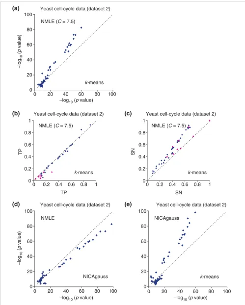
Tavazoie et al. [10] applied k-means clustering to the yeast cell cycle data generated by Cho et al. [47] (dataset 2) and

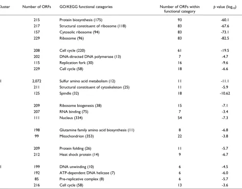
available at [54]. First they excluded two experiments due to less efficient labeling of the mRNA during chip hybridization, and then selected 3,000 genes that exhibited the greatest var-iation across the 15 remaining experiments. They generated 30 clusters with k-means clustering, after normalizing the variance of the expression of each gene across the 15 experi-ments. We used the same expression dataset and normalized the variance in the same manner, but we did not remove the two problematic experiments. Instead, we removed one experiment that made the input matrix nearly singular, which destabilizes ICA algorithms. We obtained 16 independent components, and constructed 32 clusters with our default clustering parameter (C = 7.5%). We collected functional cat-egories detected with a p value < 10-7 _{by ICA clusters only (4),} or k-means clusters only (16), or both (44). Categories cov-ered by either method but not both typically had high p val-ues. For functional categories detected by both ICA and k -means clusters, we made a scatter plot to compare the nega-tive log of the best p values of the two approaches (Figure 4a). In the majority of the functional categories ICA produced sig-nificantly lower p values. Among the functional categories with p value < 10-7 _{(or 10}-10_{), ICA outperformed}_k_-means clus-tering in 30 out of 44 (27 out of 30) cases, with a median dif-ference of 6.1 (8.9) in - log₁₀(p value). The seven most significant clusters are shown in Table 2. In Figure 4a, several functional categories are represented around the diagonal. Some of them have close connections within the GO tree with other categories for which ICA has much smaller p-values than PCA. This means that if we look at a group of similar functional categories instead of a single category, most of the groups would have smaller p values with ICA than with PCA. When adjusting the parameter C in our method (Equation 3) from four to 14, we found similar results, with ICA still significantly outperforming k-means clustering (results shown in web supplement [50]).

To understand whether ICA clusters typically outperform k -means clusters because of larger overlaps with the GO cate-gory, or because of fewer genes outside the GO catecate-gory, we defined two quantities: True Positive (TP) and Sensitivity (SN). They are determined as: TP = k/n and SN = k/f, where k is the number of genes that are shared by the functional cat-egory, the cluster n is the number of genes within the cluster that are in any functional category and f is the number of genes within the functional category that appear in the microarray dataset. For all functional categories appeared in

Comparison of linear ICA (NMLE), nonlinear ICA with Gaussian RBF kernel (NICAgauss), and PCA, on the yeast cell cycle spotted array data (dataset 1)

Figure 2 (see previous page)

Comparison of linear ICA (NMLE), nonlinear ICA with Gaussian RBF kernel (NICAgauss), and PCA, on the yeast cell cycle spotted array data (dataset 1). For each functional category within GO and KEGG, the value of -log₁₀(p value) with the smallest p value from one method is plotted against the corresponding value from the other method. (a) Gene clusters based on the linear ICA components are compared with those based on PCA when C for PCA is fixed to its optimal value 37.5. (b) Gene clusters based on the linear ICA components are compared with those based on PCA with different values of C. (c) Gene clusters based on the nonlinear ICA components are compared with those based on linear ICA. (d) Gene clusters based on the nonlinear ICA components are compared with those based on PCA. Overall, nonlinear ICA performed slightly better than NMLE, and both methods performed significantly better than PCA.

[image:7.612.54.297.424.664.2]

Three independent components of the human normal tissue data (dataset 5)

Figure 3

Three independent components of the human normal tissue data (dataset 5). Each gene is mapped to a point based on the value assigned to the gene in the 14th ₍_x_{-axis), 15}th ₍_y_{-axis) and 55}th ₍_z_{-axis) independent components,}

which are enriched with liver-specific (red), muscle-specific (orange), and vulva-specific (green) genes, respectively. Genes not annotated as liver-, muscle- or vulva-specific are colored yellow.

20

Muscle-specific component

Liver-specific component

15 10 5

Vulva-specific component

0 −5 −10

−10 −5 0 5 10 15 15

10 5 0 −5

(8)

[image:8.612.56.555.85.707.2]

Figure 4 (see legend on next page)

Yeast cell-cycle data (dataset 2)

80

100

60

40

20

0

1

0

0.2

0.4

0.6

0.8

0

20

40

60

80

100

0

20

40

60

80

100

0

0.2

0.4

0.6

0.8

1

0

0.2

0.4

0.6

0.8

1

0

0.2

0.4

0.6

0.8 −

log

₁₀

(p value)

−

log

10

(

p

value)

(a)

Yeast cell-cycle data (dataset 2)

TP

SN

TP

(b)

(c)

Yeast cell-cycle data (dataset 2)

(d)

(e)

NMLE (C = 7.5)

80

comm

en

t

re

v

ie

w

s

re

ports

refer

e

d

re

sear

ch

de

p

o

si

te

d r

e

se

a

rch

interacti

o

ns

inf

o

rmation

Figure 4a, we compared TP and SN of ICA clusters with those of k-means clusters in Figure 4b and 4c, respectively. From Figure 4b and 4c, we see that ICA-based clusters usually cover more of the functional category (more sensitive), while they are comparable with k-means clusters in the percentage of the cluster's genes contained in the functional category (equally specific). We also applied nonlinear ICA to the same dataset. We first mapped the input data from the 16-dimensional input space to a 20-dimensional feature space (see Methods), found 20 independent components in the feature space and produced 40 clusters from these components. Comparison of the biological coherence of nonlinear ICA clusters to ICA clusters and to k-means clusters (Figure 4d,e) showed that overall nonlinear ICA performed significantly better than the other methods. The seven most significant nonlinear ICA clusters are shown in our web supplement [50].

Comparison of ICA with Plaid model

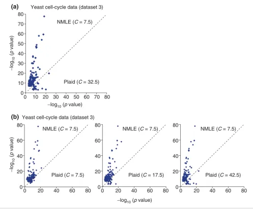
Lazzeroni and Owen [14] proposed the Plaid model for micro-array analysis. The Plaid model takes the input expression data in the form of a matrix X_ij(where i ranges over N samples and j ranges over K genes). It linearly decomposes X into component matrices, namely layers, each containing non-zero values only for subsets of genes and samples in the input X that are considered to be member genes and samples of that layer. Genes that show a similar expression pattern through a set of samples, together with those samples, are assigned to be members of that layer. Each gene is assigned a load value representing the activity level of the gene in that layer. We downloaded the Plaid software from [55], and applied it to the analysis of yeast stress data of 6,152 genes in 173 experiments (dataset 3) obtained by Gasch et al. [48] available at [56]. We imputed dataset 3 after eliminating 868 environmental stress response (ESR) genes defined by Gasch et al. [48] - because clustering of the ESR genes is trivial - and obtained 173 layers. To check the biological coherence of each layer, we grouped genes showing significant activity level in each layer into clus-ters. For each layer, we grouped the top C% of up-regulated/ down-regulated genes into a cluster. The value of C was varied from 2.5 to 42.5 with an interval of five. The setting that max-imized the average p value of the functional categories was C = 32.5, with p value of <10-20_{. (We used the most favorable} clustering coefficient C for the Plaid model, see Methods.)

We applied ICA to the dataset (5,284 genes, 173 experi-ments), after we had also eliminated the 868 ESR genes that

are easy to cluster. We found 173 independent components, constructed 346 clusters by using our default clustering parameters (C = 7.5, in Equation 3), and performed the same p value comparison of statistical significance with the Plaid model (Figure 5). Figure 5a compared ICA with the Plaid model when C is the optimal value (C = 32.5), and Figure 5b compared ICA with the Plaid model with C from 2.5 to 45. In Figure 5a, when C = 32.5, in the 56 functional categories detected by both the Plaid model and ICA with p value <10-7_, the ICA clusters had smaller p values for 51 out of 56 func-tional categories. We list the five most significant clusters from our model in Table 3. In Table 3, clusters are character-ized by functional categories related to various kinds of processes for synthesis of ATP (that is, energy metabolism), whereas clusters in Table 2 are characterized by biological events occurring during the cell cycle, most of which are cat-abolic processes consuming ATP. This result is consistent with the fact that the many cellular stresses induce ATP depletion, which induces a drop in the ATP:AMP ratio and leads to expression of genes associated with energy metabo-lism [57,58]. We also applied our approach to the dataset without removing ESR genes and the results were signifi-cantly better (see our webpage at [50]).

Comparison of ICA with topomap-based clustering

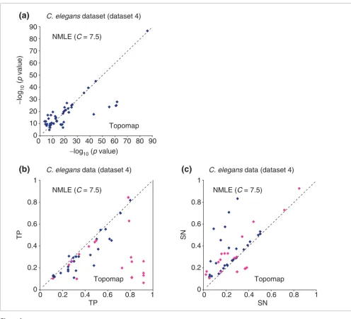
Kim et al. [8] assembled a large and diverse dataset of 553 C. elegans microarray experiments produced by 30 laboratories (available at [59]). This dataset contains experiments from many different conditions, as well as several experiments on mutant worms. Of the total, 179 of the experiments contain 11,917 gene measurements, while 374 of the experiments con-tain 17,817 gene measurements. Kim et al. [8] clustered the genes with a versatile topographical map (topomap) visuali-zation approach that they developed for analyzing this data-set. Their approach resembles two-dimensional hierarchical clustering, and is designed to work well with large collections of highly diverse microarray measurements. Using their method, they found by visual inspection 44 clusters (the mounts) that show significant biological coherence.

The ICA method is sensitive to large amounts of missing val-ues, while methods for imputing missing values are also not appropriate in such cases. We applied ICA to the 250 experiments that had missing values for < 7,000 out of the 17,661 genes, removed four experiments that make the expression matrix to be nearly singular, and generated 492

Comparison of linear ICA (NMLE), nonlinear ICA with Gaussian RBF kernel (NICAgauss), and k-means clustering on the yeast cell cycle oligonucleotide array data (dataset 2)

(10)

clusters by using our default parameters. In total, 333 GO and KEGG categories were detected by both ICA and topomap clusters with p values <10-7 _{(Figure 6). Categories covered by} either method, but not both, typically had high p values. We observe that the two methods perform very similarly, with most categories having roughly the same p value in the ICA and in the topomap clusters. The topomap clustering approach performs slightly better in a larger fraction of the categories. Still, we consider this performance a confirmation that ICA is a widely applicable method that requires minimal training, as in this case the missing values and high diversity of the data make clustering especially challenging.

We also carried out a comparison of the TP and SN quantities. For all functional categories that appeared in Figure 6a, we compared TP and SN of ICA clusters with those of topomap-driven clusters in Figure 6b and 6c, respectively. Again, typically, ICA clusters cover more genes from the functional category than the corresponding topomap clusters.

[image:10.612.62.557.118.504.2]

Comparison of different linear and nonlinear ICA algorithms We tested six linear ICA methods: Natural Gradient Maxi-mum Likelihood Estimation (NMLE) [28,29]; Joint Approximate Diagonalization of Eigenmatrices (JADE) [30]; Fast Fixed Point ICA with three decorrelation and Table 2

The seven most significant linear ICA clusters from the yeast cell cycle data (Dataset 2)

Cluster Number of ORFs GO/KEGG functional categories Number of ORFs within

functional category

p value (log₁₀)

1 215 Protein biosynthesis (175) 93 -60.1

217 Structural constituent of ribosome (118) 83 -67.6

157 Cytosolic ribosome (94) 83 -73.1

229 Ribosome (96) 83 -82.5

5 208 Cell cycle (220) 61 -19.5

202 DNA-directed DNA polymerase (13) 7 -4.7

115 Replication fork (30) 16 -9.6

229 Cell cycle (58) 18 -6.6

11 2,072 Sulfur amino acid metabolism (12) 11 -11.1

211 Structural constituent of cytoskeleton (25) 11 -5.9

125 Spindle (32) 18 -10.62

9 209 Ribosome biogenesis (38) 15 -7.1

207 RNA binding (75) 7 -3.4

111 Nucleus (334) 54 -7.3

7 198 Glutamine family amino acid biosynthesis (11) 8 -6.8

99 Mitochondrion (353) 22 -3.8

3 209 Protein folding (26) 11 -5.7

212 Heat shock protein (14) 9 -6.7

11 199 DNA unwinding (10) 6 -4.5

192 ATP-dependent DNA helicase (7) 6 -6.0

85 Pre-replicative complex (8) 6 -5.7

216 Cell cycle (58) 13 -3.6

The cluster IDs are shown, where cluster Ci,1in Equation 3 is denoted by 2i-1 and a cluster Ci,2 is denoted by 2i. The number of genes in the cluster

that have at least one annotation in GO or KEGG are listed along with the functional category with the smallest p-value among those in each annotation system. Four annotation systems are used: biological process (GO), molecular function (GO), cellular component (GO) and KEGG. Numbers in parentheses show the number of genes within the functional category that are present in the microarray data. Functional categories with p-values higher than 10-3 _{are discarded, and those with values higher than 10}-7 _{are not considered to be significant. The number of genes shared}

(11)

comm

en

t

re

v

ie

w

s

re

ports

refer

e

d

re

sear

ch

de

p

o

si

te

d r

e

se

a

rch

interacti

o

ns

inf

o

rmation

nonlinearity approaches (different measures of non-Gaussi-anity: FP, FPsym and FPsymth) [31]; and Extended Informa-tion MaximizaInforma-tion (ExtIM) [32]. We also tested two variations of nonlinear ICA: Gaussian radial basis function (RBF) kernel (NICAgauss) and polynomial kernel (NICA-poly). For each dataset, we compared the biological coherence of clusters generated by each method. Among the six linear ICA algorithms, NMLE performed well in all datasets. Among both linear and nonlinear methods, the Gaussian kernel non-linear ICA method was the best in datasets 1 and 2, the poly-nomial kernel nonlinear ICA method was best in dataset 5. NMLE, FPsymth and ExtM were best in the large datasets, 3 and 4. In Figure 7, we compare the NMLE method with three other ICA methods. We show the remaining comparisons in

our web supplement [50]. Overall, the linear ICA algorithms consistently performed well in all datasets. The nonlinear ICA algorithms performed best in the small datasets, but were unstable in the two largest datasets.

The Extended Infomax ICA algorithm [32] can automatically determine whether the distribution of each source signal is super-Gaussian, with a sharp peak at the mean and long tails (such as the Laplace distribution), or sub-Gaussian, with a small peak at the mean and short tails (such as the uniform distribution). Interestingly, the application of Infomax ICA to all the expression datasets uncovered no source signal with sub-Gaussian distribution. A likely explanation is that the microarray expression datasets are mixtures of

[image:11.612.55.552.90.505.2]

super-Comparison of linear ICA (NMLE) with the Plaid models, on the yeast stress spotted array dataset (dataset 3)

Figure 5

Comparison of linear ICA (NMLE) with the Plaid models, on the yeast stress spotted array dataset (dataset 3). For each GO and KEGG functional category, the largest -log₁₀(p value) within clusters from one method is plotted against the corresponding value from the other method. (a) Gene clusters based on the NMLE components are compared with those based on the Plaid model when C for the Plaid model is fixed to its optimal value 32.5. (b) Gene clusters based on the linear ICA components are compared with those based on the Plaid model with different values of C.

Yeast cell-cycle data (dataset 3)

Yeast cell-cycle data (dataset 3) 80

60 70

40 50

20

10 30

0

80

60

40

20

0

0 10 20 30 40 50 60 70 80

0 20 40 60 80

80

60

40

20

0

0 20 40 60 80

80

60

40

20

0

= 7.5) NMLE (

C

= 7.5) NMLE (

C

= 7.5)

Plaid (

C

= 32.5)

Plaid (

C

= 7.5) Plaid (

C

= 17.5) Plaid (

C

= 42.5)

(a)

(12)

Gaussian sources rather than of sub-Gaussian sources. This finding is consistent with the following intuition: underlying biological processes are super-Gaussian, because they affect sharply the relevant genes, typically a fraction of all genes (long tails in the distribution), and leave the majority of genes relatively unaffected (sharp peak at the mean of the distribution).

There have been several empirical comparisons of ICA algo-rithms using various real datasets [27,60]. Even though many of the ICA algorithms have close theoretical connections, they often reveal different independent components in real world problems. The reasons for such discrepancies are usually

[image:12.612.57.558.123.491.2]

deviations between the assumed ICA model and the underly-ing behavior of real data. Discrepancies can often result from noise or wrong estimation of the source distributions. Such factors affect the convergence of each ICA algorithm differ-ently, and therefore it is useful to apply several different ICA algorithms [27]. In our case, overall, the different ICA algo-rithms perform similarly. NMLE, ExtIM, and FPsymth algorithms yielded similar results except in dataset 2 where NMLE performed best. Interestingly, dataset 2 is the only one in this comparison where the data comes from oligonucle-otide microarrays (Affymetrix), where the distribution is highly unbalanced and required application of variance nor-malization (see Methods).

Table 3

The six most significant linear ICA clusters from the yeast in various stress conditions data (Dataset 3)

Cluster Number of ORFs GO and KEGG functional category Number of ORFs within

functional category

p-value (log₁₀)

17 378 Protein biosynthesis (181) 76 -37.3

407 Structural constituent of ribosome (73) 63 -57.8

225 Mitochondrion (286) 137 -77.7

423 Translation (76) 32 -15.5

15 346 Amino acid and derivative metabolism (84) 58 -47.0

379 Oxidoreductase (141) 39 -11.9

423 Metabolism of other amino acids (62) 26 -12.7

1 363 TCA intermediate metabolism (19) 18 -18.9

381 Oxidoreductase (141) 52 -22.1

198 Mitochondrion (286) 77 -22.9

421 Oxidative phosphorylation (137) 35 -24.2

65 377 Protein catabolism (123) 35 -11.1

377 Threonine endopeptidase (30) 20 -15.1

194 26S proteasome (41) 26 -18.2

423 Proteasome (32) 21 -15.5

61 375 Main pathways of carbohydrate metabolism (51) 27 -16.5

395 Transporter (218) 37 -4.8

184 Cytosol (125) 32 -9.1

421 Glycolysis/gluconeogenesis (36) 24 -17.9

75 386 Cell-cell fusion (90) 32 -12.8

390 Transmembrane receptor (14) 6 -3.3

189 External protective structure (66) 16 -4.3

The cluster IDs are shown where cluster C_i,1in Equation 3 is denoted by 2i-1 and a cluster C_i_,2is denoted by 2i. The number of genes in the cluster that have at least one annotation in GO or KEGG are listed, along with the functional category with the smallest p-value among those in each annotation system. Numbers in parentheses show the number of genes within the functional category that are present in the microarray data. Functional categories with p-values higher than 10-3 _{are discarded, and those with values higher than 10}-7 _{are not considered to be significant. The}

number of genes shared by the cluster and the functional category is shown with the log10 of the p-values corresponding to each functional category

(13)

comm

en

t

re

v

ie

w

s

re

ports

refer

e

d

re

sear

ch

de

p

o

si

te

d r

e

se

a

rch

interacti

o

ns

inf

o

rmation

Discussion

ICA is a powerful statistical method for separating mixed independent signals. We proposed applying ICA to decom-pose microarray data into independent gene expression pat-terns of underlying biological processes and to group genes into clusters that are mutually non-exclusive with statistically significant functional coherence. Our clustering method out-performed several leading methods on a variety of datasets, with the added advantage that it requires setting only one

parameter, namely the percentage ranking C beyond which a gene is considered to be associated with a component's clus-ter. We observed that performance was not very sensitive to that parameter, suggesting that ICA is robust enough to be used for clustering with little human intervention. The empir-ical performance of ICA in our tests supports the hypothesis that statistical independence is a good criterion for separating mixed biological signals in microarray data.

[image:13.612.54.550.83.533.2]

Comparison of linear ICA (NMLE) versus topomap-based clustering on the C. elegans spotted array dataset (dataset 4)

Figure 6

Comparison of linear ICA (NMLE) versus topomap-based clustering on the C. elegans spotted array dataset (dataset 4). For each functional category within GO and KEGG, the value of -log₁₀(p value) with the smallest p value from NMLE is plotted against the corresponding value from the topomap method. (a) Gene clusters based on the NMLE components are compared with those based on the Topomap method. The two methods performed comparably, as most points of low p values fall on the x = y axis. (b) TP (True Positives) of functional categories from gene clusters based on the NMLE components are compared with those of functional categories from gene clusters based on the topomap method. Functional categories for which clusters from NMLE have larger p values than those from topomap method are colored in purple. (c) SN (Sensitivity) of functional categories from gene clusters based on the linear NMLE and topomap clusters. Functional categories corresponding to the ones in purple in Figure 6b are colored in purple.

C. elegans

dataset (dataset 4)

80 90

60 70

40 50

20 30

0 10

1

0 0.2 0.4 0.6 0.8

0 10 20 30 40 50 60 70 80 90

0 0.2 0.4 0.6

TP

0.8 1

−log10 (

p

value)

−

log

10

(

p

value)

TP

1

0 0.2 0.4 0.6 0.8

0 0.2 0.4 0.6

SN

0.8 1

SN

NMLE (

C

= 7.5)

Topomap

NMLE (

C

= 7.5)

Topomap

NMLE (

C

= 7.5)

Topomap

(a)

C. elegans

data (dataset 4)

(14)

[image:14.612.59.557.83.707.2]

Figure 7 (see legend on next page) 60

50

40

30

20 10

80 100

60

40

20

0

80

60

40

20

0 0

60

50

40

30

20

0 10 20 30 40 50

0 20 40 60 80

80

60

40

20

0

0 20 40 60 80

80

60

40

20

0

0 20 40 60 80

80

60

40

20

0

0 20 40 60 80

80

60

40

20

0

0 20 40 60 80

80

60

40

20

0

0 20 40 60 80

100 80 100

60

40

20

0

0 20 40 60 80 100

80 100

60

40

20

0

0 20 40 60 80 100

60 0 10 20 30 40 50 60 0 10 20 30 40 50 60

10

0

60

50

40

30

20 10

0 NMLE

C. elegans data (dataset 3)

NMLE NMLE

ExtlM FPSymth NICApoly

NMLE NMLE NMLE

−log10 (p value)

−

log

10

(

p

(15)

comm

en

t

re

v

ie

w

s

re

ports

refer

e

d

re

sear

ch

de

p

o

si

te

d r

e

se

a

rch

interacti

o

ns

inf

o

rmation

Linear ICA models a microarray expression matrix X as a lin-ear mixture X = AS of independent sources. ICA decomposi-tion attempts to find a matrix W such that Y = WX = WAS recovers the sources S (up to scaling and permutation of the components). The three main mathematical conditions for a solution to exist are [42]: the number of observed mixed sig-nals is larger than, or equal to the number of independent sources, that is, N = M in Equation 1; the columns of the mix-ing matrix A are linearly independent; and there is, at most, one source signal with Gaussian distribution. In microarray analysis, the first condition may mean that when too few sep-arate microarray experiments are conducted, some of the important biological processes of the studied system may col-lapse into a single independent component. If the number of sources is known to be smaller than the number of observed signals, PCA is usually applied prior to ICA, to reduce the dimension of the input space. Because we expect the true number of concurrent biological processes inside a cell to be very large, we attempted to find the maximum number of independent components in our tests, which is equal to the rank of X. We also experimented with adjusting the number of independent components by randomly sampling a certain number of experiments and by using dimensional reduction using PCA for the datasets 1, 2 and 3 (results shown in the web supplement at [50]). Both random sampling and PCA dimensional reduction led to worse performance in terms of p values as the number of dimensions decreased. The main conclusion that we can draw from this drop in performance is to exclude a scenario where a small number of linearly mixing independent biological processes drove the expression of most genes in these datasets. The second condition, that the columns of the mixing matrix A are linearly independent, is easily satisfied by removing microarray experiments that can be expressed as linear combinations of other experiments, that is, those that make the matrix X singular. The third con-dition, that there is, at most, one source signal with Gaussian distribution, is reasonable for analyzing biological data: the most typical Gaussian source is random noise, whereas biological processes that control gene expression are expected to be highly non-Gaussian, sharply affecting a set of relevant genes, and leaving most other genes relatively unaffected. Moreover, the ability of ICA to separate a single Gaussian component may prove ideal in separating the experimental noise from expression data. This is a topic for future research.

ICA is a projection method for data analysis, but it can be interpreted also as a model-based method, where the under-lying model explains the gene levels at each condition as

mixtures of several statistically-independent biological proc-esses that control gene expression. Moreover, ICA naturally leads to clustering, with each gene assigned to the clusters that correspond to independent components where the gene has a significantly high expression level. An advantage of ICA-based clustering is that each gene can be placed in zero, one or several clusters.

ICA is very similar to PCA, as both methods project a data matrix into components in a different space. However, the goals of the two methods are different. PCA finds the uncorrelated components of maximum variance, and is ideal for compressing data into a lower-dimensional space by removing the least significant components. ICA finds the sta-tistically independent components, and is ideal for separating mixed signals. It is generally understood that ICA recovers more interesting (that is, non-Gaussian) signals than PCA does in the financial time series data [25]. If the input com-prises a mixture of signals generated by independent sources, independent components are close approximates of the indi-vidual source signals; otherwise, ICA is the projection-pursuit technique that finds the projection of the high-dimensional dataset exhibiting the most interesting behavior [44]. Thus, ICA can be trusted to find statistically interesting features in the data, which may reflect underlying biological processes.

We applied a new method for performing nonlinear ICA, based on the kernel trick [37] that is usually applied in Sup-port Vector Machine (SVM) learning [61]. Our method can deal with more general nonlinear mixture models (generalized post-nonlinear mixture models), and reduces the computation load so as to be applicable to larger datasets. Using nonlinear ICA we were able to improve performance in the three smaller datasets. However, the algorithm was still unstable in the two larger datasets. Using a Gaussian kernel, the method performed very poorly in these datasets; using a polynomial kernel, it performed comparably to linear ICA. Overall we demonstrated that nonlinear ICA is a promising method that, if applied properly, can outperform linear ICA on microarray data.

In nonlinear mixture models, the nonlinear mapping f(.) rep-resents complex nonlinear relationships between biological processes s₁...s_Mand gene expression data x_1...x_N. In our non-linear ICA algorithm, the nonnon-linear step based on kernel method is expected to map the data x₁...x_Nfrom the input space to a higher dimensional feature space where these non-linear operations become non-linear so that the relationship

Comparison of NMLE with other ICA approaches

(16)

between biological processes s₁...s_Mand the mapped data

Ψ(x₁),..., Ψ(x_N) becomes linear. Kernel-based nonlinear ping has many advantages compared to other nonlinear map-ping methods because it is versatile enough to cover a wide range of nonlinear operations, and at the same time reduces the computational load drastically [34]. One challenge in gen-eral is to choose the best kernel for a specific application [62,63]. A common practice is to try several different kernels, and decide on the best one empirically [3,34]. Finding which kernels best model observed nonlinear gene interactions is a direction for future research.

The linear mixture model that we proposed has the advantage of simplicity - it is expected to perform well in finding first-order features in the data, such as when a single transcription factor up-regulates a given subset of genes. Nonlinear ICA may prove capable of capturing multi-gene interactions, such as when the cooperation of several genes, or the combination of presence of some genes and absence of others, is necessary for driving the expression of another set of genes. In future research, we will attempt to capture such interactions with nonlinear modeling, and to deduce such models from the components that we obtain with nonlinear ICA. Currently our ICA model does not take into account time in experiments such as the yeast cell cycle data. A direction for future research is to incorporate a time model in our approach, whenever the microarray measurements represent successive time points.

It has been suggested that ICA be used for projection pursuit (PP) problems [64] where the goal is to find projections containing the most interesting structural information for visualization or linear clustering. ICA is applicable in this context because directions onto which the projections of the

data are as non-Gaussian as possible are considered interest-ing [60]. Unlike the BSS problem, in the projection pursuit context inputs are not necessarily modeled as linear mixtures of independent signals. In dataset 5, we can see difference between ICA and PCA in finding interesting structures. Using a previous version of dataset 5 containing 40 out of the 59 samples, Misra et al. [19] constructed a scatter plot illustrat-ing the two most dominant principal components. On that plot, there were three linearly structured clusters of genes, each turning out to be related to a tissue-specific property. Two of them were not aligned with any principal components. The corresponding plot derived by ICA in Figure 3 shows that the directions of the three most dominant independent com-ponents are exactly aligned with the linear structures of genes so that we can say that each component corresponds to a tis-sue sample. It is known that by applying ICA, separation can be achieved along a direction corresponding to one projec-tion, which is not the case with PCA [60]. Nonlinear ICA can similarly be understood to be a PP method that finds nonlinear directions that are interesting in the sense of form-ing highly non-Gaussian distributions.

[image:16.612.56.559.117.281.2]

In practice, microarray expression data usually contain miss-ing values and may have unsymmetrical distribution. In addi-tion, there maybe false positives due to experimental errors (for example, weak signal, bad hybridization and artifact) and intrinsic error caused by dynamical fluctuations in photoelec-tronics, image processing, pixel-averaging, rounding error and so on. In the datasets we used in the current analysis, missing values comprise 1.427%, 3.187% and 8.55% for data-sets 1, 3 and 4, respectively. The datadata-sets have undergone log transform normalization so that equivalent fold changes in either direction have the same absolute value. Moreover, they do not have symmetrical distribution (shown in the web Table 4

Methods for performing ICA that we compared

Algorithm Variations Abbreviation Description Reference Software

Natural Gradient Maximum Likelihood Estimation

- NMLE Natural gradient is applied to MLE for

efficient learning

[28,29] [72]

Extended Information Maximization

- ExtIM NMLE for separating mix of super-

and sub-Gaussian sources

[32] [73]

Fast Fixed-Point Kurtosis with deflation FP Maximizing non-Gaussianity [31] [74]

Symmetric orthogonalization Fpsym