M a c hi n e l e a r n i n g a n d D S P
a l g o ri t h m s fo r s c r e e n i n g of
p o s si bl e o s t e o p o r o si s u si n g
e l e c t r o ni c s t e t h o s c o p e s
S c a n l a n , J, Li, FF, U m n o v a , O, R a k o c zy, G a n d Löv ey, N
h t t p :// dx. d oi.o r g / 1 0 . 1 1 4 5 / 3 2 8 8 2 0 0 . 3 2 8 8 2 1 5
T i t l e
M a c hi n e le a r ni n g a n d D S P a l g o r i t h m s fo r s c r e e n i n g of
p o s si bl e o s t e o p o r o si s u si n g el e c t r o n i c s t e t h o s c o p e s
A u t h o r s
S c a n l a n , J, Li, FF, U m n o v a , O, R a k o c zy, G a n d Löv ey, N
Typ e
C o nf e r e n c e o r Wo r k s h o p I t e m
U RL
T hi s v e r si o n is a v ail a bl e a t :
h t t p :// u sir. s alfo r d . a c . u k /i d/ e p ri n t/ 4 8 8 0 3 /
P u b l i s h e d D a t e
2 0 1 8
U S IR is a d i gi t al c oll e c ti o n of t h e r e s e a r c h o u t p u t of t h e U n iv e r si ty of S alfo r d .
W h e r e c o p y ri g h t p e r m i t s , f ull t e x t m a t e r i al h el d i n t h e r e p o si t o r y is m a d e
f r e ely a v ail a bl e o nli n e a n d c a n b e r e a d , d o w nl o a d e d a n d c o pi e d fo r n o
n-c o m m e r n-ci al p r iv a t e s t u d y o r r e s e a r n-c h p u r p o s e s . Pl e a s e n-c h e n-c k t h e m a n u s n-c ri p t
fo r a n y f u r t h e r c o p y ri g h t r e s t r i c ti o n s .
Machine learning and DSP Algorithms for Screening of
Possible Osteoporosis Using Electronic Stethoscopes
Jamie Scanlan
Acoustics Research Centre University of Salford, M5 4WT, UK+44 (0) 752 723 6432
*[email protected]
Gyorgy Rakoczy
Acoustics Research Centre University of Salford, M5 4WT, UK+44 (0) 773 690 8638
[email protected]
Francis F. Li
Acoustics Research Centre University of Salford, M5 4WT, UK+44 (0) 161 295 5462
[email protected]
Olga Umnova
Acoustics Research Centre University of Salford, M5 4WT, UK+44 (0) 161 295 4666
[email protected]
Nóra Lövey
Rheumatology Department Warrington Hospital, WA5 1QG, UK+44 (0) 192 563 5911
[email protected]
ABSTRACT
Osteoporosis is a prevalent but asymptomatic condition that affects a large population of the elderly, resulting in a high risk of fracture. Several methods have been developed and are available in general hospitals to indirectly assess the bone quality in terms of mineral material level and porosity. In this paper we describe a new method that uses a medical reflex hammer to exert testing stimuli, an electronic stethoscope to acquire impulse responses from tibia, and intelligent signal processing based on artificial neural network machine learning to determine the likelihood of osteoporosis. The proposed method makes decisions from the key components found in the time-frequency domain of impulse responses. Using two common pieces of clinical apparatus, this method might be suitable for the large population screening tests for the early diagnosis of osteoporosis, thus avoiding secondary complications. Following some discussions of the mechanism and procedure, this paper details the techniques of impulse response acquisition using a stethoscope and the subsequent signal processing and statistical machine learning algorithms for decision making. Pilot testing results achieved over 80% in detection sensitivity.
CSS Concepts
•
Applied computing~Health informatics
•
Computing methodologies~Machine learning
•
Keywords
Osteoporosis; diagnosis; screening test; impulse response, signal processing, stiffness; resonant frequencies, machine learning; electronic-stethoscopes patient screening acoustic signals; impulse response.
1.
INTRODUCTION
Bone undergoes a regeneration process where collagen and mineral is added then removed for remodelling. As the skeleton develops more bone is added than is being taken away. The
process eventually stabilises and the bone mass remains constant. If however, more bone is removed than added, akin to skeletal bio-corrosion, we have a condition called osteoporosis. Osteoporosis literally means ‘porous bone’ and describes a period of largely asymptomatic bone loss leading to skeletal fragility and increased risk of fracture. One in three women and one in five men over the age of 50 will break a bone attributed to osteoporosis according to well known public surveys. Osteoporosis affects more than 75 million people in the Europe, United States and Japan, being the cause of more than 8.9 million fractures annually worldwide. It is well established that early diagnosis and treatments are the key to prevent further complications and fractures. The lack of a simple and practical diagnostic method for screening has been identified as a major cause of delayed diagnosis and poor prognosis.
The paper proposes a vibroacoustic method, using the bone’s ‘impulse response’, to estimate the likelihood if a person is sustaining osteoporosis. It is based on bio-mechanical theories, a clinically collected database and computer learning algorithms. A clinician taps a specific part of a patient’s tibia bone with a Taylor reflex hammer, an electronic stethoscope picks up the induced sound at the midpoint and/or the distal end of the tibia. The signal is transmitted via a Bluetooth datalink to a computer for further signal processing and gives a verdict on the patient’s diagnosis. The hypothesis is that the bone’s bending stiffness, mass, and densities can be interpreted from its resonant frequencies with some necessary assumptions. The decision to suggest that a patient might have osteoporosis is based on machine learning. The algorithm looks for common features in the time-frequency domain from a good number of acoustical examples of normal and osteoporotic subjects, then generalises the knowledge for decision making.
2.
BACKGROUND AND RATIONALE
2.1
Background
the patient has osteoporosis. However the BMD is not an accurate or reliable measure of the bone’s strength and can only imply bone quality [3, 4]. While there is a connection between low BMD (t-score) and higher fracture risk, a low BMD is not a prerequisite to a low trauma fracture. Other methods such as Quantitative ultrasound (QUS) and recently the more direct Mechanical Response Tissue Analysis (MRTA) have found their uses and been studied as alternatives, but the former relies on the speed of sound transmission, again a proxy measure of stiffness, while MRTA is still yet to find wider clinical use [5,6].
Research into bio-mechanics investigated the vibro-acoustic response as a means of describing the quality of bone macrostructure. The objective as reported from the literature was to find a parameter which would correlate strongly with the condition of the bone and therefore could be used as an index for diagnosis. The lowest resonant frequency found some limited adoption as a parameter, but this has been questioned as the dynamics of the whole limb becomes better understood.
Stethoscopes have been used for auscultating the sound transmitted through bones by tapping the body and listening through the chest [7]. This required a high level of practice and experience to identify the sound of a diseased bone, and could be too holistic for general diagnosis. But the potential of using a stethoscope for auditioning the vibro-acoustic response instead of typical laboratory equipment is explored further in this paper: directly listening to the bone’s vibration in question rather than through the chest.
Machine learning was used in the diagnosis of osteoporosis from the tibia’s lowest resonant frequency and other physiological information of patients [8]. The algorithm mimics the already-established fracture prediction algorithm ‘FRAX’ rather than signal processing and information extraction. The only physical measure adopted was the lowest resonant frequency, which was known to be inadequate to reliably determine the quality and fragility of bones. The complex set-up and procedure, including an accelerometer, a dedicated charge amplifier and an analogue to digital converter, and the use of an impact hammer as described in [8], are unlikely to find adoption for front-line screening tests.
2.2
Rationale
2.2.1
Bone Structure
Vibration analysis has found common use in engineering to characterize certain properties of a structure. Several parameters relevant to bone quality, such as its stiffness/mass ratio, its elastic modulus and natural modes of vibration, are contained in its impulse responses. In particular, the resonances are related to the stiffness/mass ratio.
Bone is a complex anisotropic structure which is made of two main phases: a surface layer of calcium and an internal network structure (trabeculae) [4]. The trabeculae are arranged in plates along the bone to give strength in typical load directions. Its modes of vibration will therefore depend on their axis and type, each with a different stiffness. The complexity and diversity in the bony structures of individuals make accurate mathematical modelling and analytical solutions of governing equations extremely difficult. Using the machine learning approach for this type of complex problem is a sensible choice if a large number of examples can be collected.
2.2.2
Bio-Mechanical Research
Research into bone vibration in the 1970s suggested that the lowest fundamental frequency was related to the bending stiffness of the bone, and therefore the quality of the bone [9, 10]. This is in line with what is found in a simple rod model: the square root of the stiffness/mass ratio will give the lowest resonant frequency of the object:
(1)
where (N/m) is the stiffness of the bone, (kg) is the mass and (Hz) is the fundamental frequency. Therefore a drop in stiffness will reduce the frequency. While having osteoporosis does result in reduced stiffness of the bone, it also removes mass from the bone. Such a decrease in the mass will counter-act on the reduction of the lowest resonant frequency. Fortunately, much of the research indicated that lowered resonant frequencies and shifting in modal frequencies’ distribution are often associated with osteoporosis, though the strict proportional relation between the resonant frequency and the square root of stiffness does not hold, due to the fact that mass is a yet another dependent variable [11,12,13,14,15].
2.2.3
Machine Learning vs. Analytical Model
Attempts have been made to derive an analytical model of the bone vibration response by using slender beam theory and hollow cylinders to predict the modal shapes and frequencies. These have been followed by FE (finite element) models investigating parameter changes and their effect on the bone response [16]. There has been moderate agreement with experimental results with the assumption that the bone is isotropic. However it is clear in reality that bone is highly anisotropic, leading to over-simplified results.
Bone, when impacted on, sustains different waves at any moment in time, but it is difficult to be certain which wave shape relates to which modal frequency from a frequency response. Therefore using a purely analytical or empirical model is not sufficient to made accurate predictions on the extent of osteoporosis. Instead, a statistical machine learning algorithm can be used where analytical solutions are difficult to obtain or where laboratory replication is impractical. With a large enough dataset the algorithms might be trained to learn from examples with a “teacher” (senior doctors’ diagnosis) and generalise the acquired knowledge to correctly diagnose cases not previously included in the training. Further inspired by the fact that one can tap on a piece of furniture to evaluate its solidity from the sound, it is therefore reasonable to hypothesize that an audition approach can train a computer algorithm to listen to the tapping sound from the bone in question and make a statement on the quality of the bone.
2.2.4
Stethoscope
software [18]. It has found more adoption in clinical use than the other models, and 3M offers a software development kit (SDK) which allows for future expansion of the capabilities of the device. While the market for electronic stethoscopes is still small and fractured, these devices are the only way of being able to use the digital signal processing methods to detect signals and problems that would be very difficult to find by auralization alone.
3.
THE METHOD
3.1
Reflex Hammer and Stethoscope Method
The patient’s limb is held in the supine position, supported on furniture or other height. The Taylor hammer is used to tap the tibial tubercle of the tibia. The stethoscope is placed in the anterior border, where the bone is deemed most flat and closet to the surface. The practitioner then taps with moderate force (about 10-30 N) at the impact site with about 1 s gap in between consecutive taps. The number of taps and the total duration are not important, but for this project 8 knocks were recorded in a 15 second recording.
The stethoscope is connected to a computer running StethAssist software via Bluetooth. The software primes the stethoscope to record. The stethoscope has digital filters to emulate the bell and diaphragm of an acoustic stethoscope [18]. For the purposes of the listening session, the third filter option: “extended range” is used. This can be assumed to be the ‘original’ signal which ranges from 20 Hz - 1 kHz. Once the session is complete, the recording is exported as an audio file with the extended range filter enabled to be used inside MATLAB. The exported file is a .wav format audio file with a sample rate of 4 kHz.
[image:4.612.321.553.242.521.2]Previous research had used impact hammers and accelerometers to study the bone response, e.g. [8]. Our Taylor hammer and stethoscope must be able to repeat these findings and show equivalency. To compare the two sensors, the stethoscope was placed onto a metal plate, with an accelerometer (B&K Type 4507) underneath at the same point connected to a converter into vibro-acoustics software (B&K PULSE LabShop). This was to confirm that given a common medium, the two receivers will respond the same. Their placement is shown in figure 1. An impact hammer (B&K Type 8206) struck the plate and the input force was recorded. The stethoscope recorded the audio output while the vibration software gave the frequency response function of the accelerometer. The recordings were passed through a MATLAB script and compared with the results from Pulse. The results show the same resonant peaks found in the frequency response function from the Pulse software occurred in the FFT of the recordings. In terms of magnitude response some necessary equalisation is needed as detailed in the next section.
Figure 1. Stethoscope and accelerometer for equivalency tests.
3.2
Reflex Hammer/Stethoscope Response
The reflex hammer and electronic stethoscope are not ideal impact source and perfect transducer. The Taylor hammer does not produce a perfect impact with a flat spectrum because of its semi-solid rubber construction, effectively imposing a low-pass filtering effect. Combined with the damping effect of the soft tissue, this reduces the useful region down to a few kilohertz, which should still excite and pick up vibration modes of interest for this study.
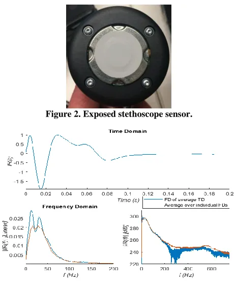
The stethoscope is built on a piezoelectric transducer behind a thin rubber cover as shown in figure 2 [17]. The frequency response of the stethoscope itself shows a rolling-off starting at 600 Hz. It also shows resonances in the LF region, from 10 - 40 Hz. The impulse response shown in figure 3 is acquired from tapping the rubber cover of the stethoscope with the Taylor’s hammer directly. This represnets the intrinsic artefects of the signal chain, and if desirable, can be de-convolved out.
Figure 2. Exposed stethoscope sensor.
Figure 3. Reflex hammer-stethoscope's responses.
3.3
De-convolution or Equalization
The recorded stethoscope signal is the convolution of the response of the bone, the soft tissue as well as all the devices in the signal chain:
(2) where is the recorded signal, is the bone response, is the
soft tissue response, is the Taylor hammer and is the
stethoscope response.
To isolate the sound of the bone and soft tissue, the response of the signal chain has to be removed. This can be done by taking an impulse response of the devices in the chain, either separately or all as one, and filtering their responses in the frequency domain.
[image:4.612.55.262.571.698.2]
(4) This can be simplified by grouping the signals into:
(5)
where represents the while limb (bone and soft tissue) and is the signal chain (the hammer and stethoscope).The filtering will therefore leave only the modal response of the bone in vivo with the muscle and soft tissue attached. This should in theory remove the influence of the signal chain entirely, but if the response of the signal chain is non-linear, then some artefacts will still remain in the recording. The muscle and soft tissue’s effect on the bone’s vibration response would also be unchanged, owing to its connection with the bone itself.
3.4
Dataset
[image:5.612.315.564.156.232.2]The dataset contains a series of recordings collected in 2016 from 30 patients by Rakoczy following the method described in Section 3.1. A summary is in given in Table 1. Each patient was recorded 5 times, with 8 knocks in each recording. These recordings are exported and put through MATLAB scripts developed for this project to perform time domain gating and alignment and give further frequency domain and cepstrum domain representations. The detail of that data analysis is detailed in Section 4. The data structure of the dataset is described in Table 2. Of course, senior doctors’ diagnoses are annotated and used as the teacher values.
Table 1. Population Statistics
Parameter Mean [Min, Max]
Age 66.25 [51,93] DXA -0.95 [-3.3, 0.5] Weight 68.33 [46,93]
Height 161 [152,176]
Table 2: Dataset parameters
Parameter Size Unit
IR Sample Length 800 samples FFT Window Length 8192 points FFT Output Spectra Size 100 points MFCC Window Length 0.03 seconds MFCC Window Overlap 0.02 seconds MFCC Total 378 points
4.
SIGNAL PRE-PROCESSING
4.1
Alignment and Normalization
The recordings are imported into a MATLAB script to isolate the impulse responses (IR). The data is normalized and any offset removed. Because of the noisy nature of the recordings, the gradient and the Hilbert amplitude envelope of the waveform are separately used to isolate the impulses from the files. The gradient is used first to detect the rise of the impulse (represented as a peak in the gradient) and begins the ‘cut’ procedure to isolate it. The amplitude envelope then is used to find when the level of the signal is below the threshold when the impulse has assumed to
[image:5.612.354.512.271.394.2]end (figure 4). There are two checks to remove erroneous impulses: a peak level threshold (to remove low level impulse noises) and a peak position (to avoid early triggering). This does assume that the peak of the impulse is very soon after the zero-crossing point, which can be broken by loud impacts elsewhere near the stethoscope. Also recordings with high level of noise can cause miss-triggering or false positives. The signals are then normalized again to remove any impulse to impulse variation. An example of the time domain representation is given in figure 5.
Figure 4. Zoom of waveform (Light Blue) with gradient (Orange) and Hilbert envelope (Dark Blue)
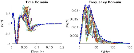
Figure 5. Individual IR with one misalignment.
4.2
Equalization and Pre-emphasis
Since machine learning will normally learn to ignore (or compensate) spectrum coloration from the stethoscope and reflex hammer, for a convenient solution the data can be left unfiltered. However, there are advantages in accuracy and speed of convergence if the influence of the stethoscope and the reflex hammer is de-convolved out as mentioned in Section 3.3. Figure 6 shows time and frequency domain responses from multiple reflex hammer impacts on the stethoscope. The maximum envelope of the spectra is used for the design of equalization filter. The reflex hammer and stethoscope system has a clear spectral rolling-off when frequency increases. A pre-emphasis high pass filter of 12dB/Oct to 24 dB/Oct starting from 63 Hz can be used as a simpler but rather effective compensation mechanism before the signal is further processed, rather than strict equalization.
[image:5.612.56.302.351.581.2] [image:5.612.324.542.581.668.2]4.3
Frequency Domain Feature Extraction
[image:6.612.93.255.226.499.2]The signals are transformed into the frequency domain.Owing to the very short duration of the impulses (800 samples) and the low sample rate, the window length is made much larger (zero padding) to increase the resolution (L = 8192). The results of the absolute spectrum are displayed in figure 7. There is a clustering of peaks in the very low frequency region, which we assume to be the resonances of the stethoscope as described previously. A second group of peaks are found at 75-110 Hz, which would agree with [8, 19]. Further along there is a cluster of much more damped peaks in the 200 - 250 Hz region, which would match the findings in much of the previous bio-mechanics literature [9, 15, 16]. Looking for sign changes in the imaginary component will confirm which peaks are true resonances of the tibia and which are noise peaks. The real and imaginary components are in figure 8.
Figure 7. Absolute frequency spectra of IR
Figure 8. Real and Imaginary parts of spectra. (Only positive values of real part is displayed).
While there is some agreement with the previous findings, there are some discrepancies in the repeatability and exact correlations. The signals from osteoporotic subjects do not show strong clustering, or are too heavily damped to be identified. Secondly the resonant frequencies do not always shift in accordance with the t-score as described by some authors. These observations suggest that the use of lowest resonant frequency alone is not reliable in detecting osteoporosis. Therefore the pattern of modal frequencies is instead used in this study.
4.4
MFCC
FFT spectral analysis uses filter bands with equal frequency bins. It is not an efficient representation for many types of audio signals requiring uneven frequency sampling. To reduce the data points and mitigate the complexity of machine learning, time-frequency domain representations, namely Mel Frequency Cepstrum Coefficients (MFCCs) are used to capture the features and
resonance patterns. The MFCCs are found popular use in speech recognition and music classification. Taking the discrete Fourier transform (FT) of a time domain signal, and then taking the inverse DFT of the logarithm of the FT spectrum to express the signal in the time-frequency domain is called the Cepstrum. For the real part of the cepstrum:
(6)
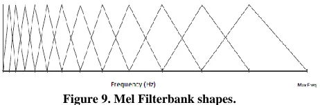
For MFCC an extra filtering stage is included after the initial FT with logarithmically spaced triangular filters, which emulate the frequency selection filters in the human ear (Figure 9). The filters are spaced on the Mel scale from psychoacoustics, which is a subjective measurement of pitch instead of linear frequency.
(7)
[image:6.612.330.561.272.348.2]The number of filters dictates the number of coefficients required to describe the energy of each filter band in time. The log energies are calculated per Mel band and are passed though a cosine transform. For this project 21 coefficients are used.
Figure 9. Mel Filterbank shapes.
[image:6.612.373.497.439.553.2]Because the IRs are so short and with many influences on the vibration response, using MFCC is a valid option with a slightly larger window. The algorithm used is the ‘mfcc.m’ function included with MATLAB 2018a, based on the “Auditory Toolbox” from Interval Research. The sum of the coefficients of each IR is given lastly in figure 10.
Figure 10. Cepstrum coefficient sum of IR. (Colour bar is clipped to increase resolution).
Wavelet analysis was considered, as like MFCC it displays complex frequency and phase interactions in the time-frequency domain. For this project MFCC was deemed to be more convenient, as it already contains the non-linear distribution of frequency filtering, weighted more towards the lower frequencies.
5.
MACHINE LEARNING
5.1
Neuron Model
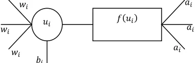
expected outputs. There are several different methods of achieving this goal (decision trees and support vector machines are examples), but one which is most popular in engineering applications is the feed-forward Artificial Neural Network (ANN). The data is processed through individual neuron models (shown in figure 11), which have several connections for inputs with weighting coefficients, sometimes with a bias offset. This is expressed as:
[image:7.612.61.253.227.289.2]
(8) where is the current neuron, is the next neuron in the next layer of the network, is the weight from the th to the th neuron, the input to that neuron and is the bias term.
Figure 11. Neuron Model: summation and activation function.
The activation function then shapes the summed and weighted inputs into a single output, either as binary logic via a threshold or as a sigmoid function for a continuous output bounded in the interval (0,1). A continuous sigmoid function is used in this study.
(9)
5.2
Multi-layer feed forward neural network
Figure 12. Neuron network model
ANNs rely on a large number of connected neuron models to deliver computational power and learning capability. A classical fully connected feed-forward network featuring two non-linear hidden layers of decreasing number of neurons, as depicted in Figure 12, is empirically found appropriate for the current study. The input layer is as large as the number of data points and has only one input per neuron. The hidden layers reduce the data and manipulate the weights to find the optimal solution. The output layer has only one neuron and a sigmoid activation function is adopted. There is no strict rule or theory prescribing the number of neurons per layer or the number of layers in the network, since the model is data driven and is highly depends on the context. For this paper the network was built with 378 neurons for the input layer, 120 for one hidden layer and 1 output neuron. Each set of MFCCs has 21 data point, 18 sets of MFCCs (acquired through moving windows with overlap) gives 18 x 21 = 378 coefficients arranged in column vector as input to the neural network.
The ANN starts from random weights; the percussion sound represented in 378 coefficients is presented at the input; the output of the network is compared with the doctor’s diagnosis (“teacher value”). The aim of training is to minimise the total square error E
as defined in Equation 10 over all training examples.
(10) where is the ANN output is teacher value m is example number.
The well established back-propagation algorithm is used for training. It updates the weights of the output layer first then onwards to the previous layers by updating the weights according to
(11)
where represents connecting weights between ith and jth
neurons, l represents the layer. Changes made to the weight matrix are determined using a chain rule:
(12)
(13) (14) where is the learning rate (step size) and:
(15)
6.
TRAINING & VALIDATION
After applying the data scrutiny algorithm, as described in Section 4.1, the training set includes 48 impulse responses and the validation set contains 46 samples that had not been encountered in training. The network is given the teacher values given by senior doctors’ diagnoses, which are generally in line with the aforementioned WHO guidelines, i.e. t-scores below -2.5 as osteoporotic (OP) (teacher value: 0); the rest are deemed OK (teacher value: 1). But some other conditions and aspects are also taken into account.
For any iterative algorithm, a stop criterion is always needed to determine when the algorithm should be terminated. A common practice is to freeze the weights when over-fitting starts to occur. It is not surprising when testing with the examples in the training set that 100% accuracy is always possible when training is left running for sufficiently long period of time. Validation of the generalization showed over 80% correct classification when stopped immediately before over-fitting occurs. The actual percentage varies slightly depending on step size and each different random start.
To evaluate the clinical usefulness of the method, it is important to find how specific and sensitive the algorithm is. This is a medical version of a hypothesis test, where there are type 1 and type 2 errors (false positives and false negatives). Specificity describes how accurate the algorithm is in detecting OK patients while reducing false negatives. Sensitivity describes the opposite: how accurate the algorithm is in detecting the OP subjects while
reducing false positives. A highly sensitive test is one which will not miss an OP patient, but perhaps at the expense of diagnosing other subjects that are not. While a highly specific test would be very strict about who is diagnosed, leaving the fewest false positives, but at the loss of some which are positive but missed. Furthermore, 3 practical stop criteria were experimented with over 12 patient cases to explore the generalisation behaviour, with a range of learning rates. Some of the validation results are detailed below.
[image:8.612.332.517.54.172.2](1) When the squared error, as in Equation 10, falls below 0.05, i.e any individual case will be rounded to the correct category. Figure 14 a) and b) give some of the results for illustration.
[image:8.612.57.245.173.491.2]Figure 14. a) Patient sensitivity result.
Figure 14. b) False negatives found in validation.
It can be observed in Figure 14 b) there is a period of rapid oscillating change in overall error. This indicates the likelihood of missing some valuable local minima, leading to poor results even at a late stage.
(2) When the algorithm reached 80% accuracy for both the OK and OP cases. This is presented in Figure 15 a) and b).
Figure 15. a) Correct diagnoses out of 3 positive patients.
Figure 15. b) Number identified as OK out of 35 IR’s.
For a medical application the possibility of false negatives is a concern. It is observed in Figure 15 b) for low learning rates the false negatives for individual IR is low in the initial stages (0 - 2 seconds run time) but once the algorithm starts to balances to reduce the false positives, the false negative rate rises. At high learning rates such as 0.5, the network rebalances at the expense of increasing false negatives for IR identification. However this does not affect the patient results, which still shows the osteoporotic patients being diagnosed as such.
[image:8.612.57.242.196.326.2](3) When the algorithm was able to correctly identify all the patients that were OK and OP. Figure 16 a) and b) give examples of this.
[image:8.612.322.498.334.452.2]Figure 16. a) Patient sensitivity result of ANN.
Figure 16. b) IR sensitivity result of ANN.
Overall, as the training error decreases, the number of patients correctly identified increases, while the number of IR correctly identified converges to stable values. The typical training time to reach the three criteria is given in Table 3.
Table 3: Typical training times for different learning rates
Learning
[image:8.612.59.244.342.465.2] [image:8.612.321.506.482.602.2] [image:8.612.61.241.565.684.2]0.3 130.52 2.31 39.17 0.2 207.18 3.03 43.33 0.1 343.41 4.14 74.87
7.
CONCLUDING REMARKS
A new method for the screening testing of osteoporosis has been developed in this paper. Using two pieces of common medical apparatus, a reflex hammer, an electronic-stethoscope, and machine learning based intelligent decision making algorithms loaded in a computer (even possible with a mobile phone), tests can be done in basic clinics by virtually any healthcare professionals, making it particularly suitable for GPs’ or primary healthcare professionals for large scale screening testing. Although typical machine learning methods are a blackbox approach to complex problems, the method proposed in this paper may be deemed as being semi-analytical, as the physical meaning for bony resonance frequencies and their distribution patterns are known to correlate to the stiffness, porosity and many other relevant physical parameters of bones. As a proof of concept pilot study, the paper only used a limited number of examples. Even so a sensitivity of 80% seems achievable. It is envisaged if a larger dataset is made available and the understanding of the bone resonance is further deepened, the proposal method has a potential to become a clinically useful one.
8.
ACKNOWLEDGEMENT &
CONTRIBUTIONS
Jamie Scanlan would like to thank Dr. Pascal Scanlan for review and medical terminology.
Contributions: Mr. Scanlan for data analysis, method implementation, reporting results; Dr. Li for direction of signal processing & machine learning; Dr. Umnova for direction of physical modelling, analysis & mechanisms; Dr. Rakoczy for instigating the reflex hammer percussion response audition research and carrying out patient data recordings; Dr. Lövey for diagnostic notation & clinical knowledge.
9.
REFERENCES
[1] Kanis, J. A. 2002. Diagnosis of osteoporosis and assessment of fracture risk. The Lancet. 359(9321), 1929-1936 [2] Kanis, J. A. WHO Study Group. 1994. Assessment of
Fracture Risk and its Application to Screening for
Postmenopausal Osteoporosis: Synopsis of a WHO Report.
Osteoporosis International. 4(6), 368-381.
[3] Kanis, J. A. Johnell, O. Oden, A. Jonsson B. De Laet, C. Dawson A. 2000. Prediction of Fracture From Low Bone Mineral Density Measurements Overestimates Risk. Bone
26(4), 387-391.
[4] Bouxsein, M. L. 2003. Mechanisms of Osteoporosis Therapy: A Bone Strength Perspective. Clinical Cornerstone Supplement 2 S13-S21.
[5] Djokoto, C. Tomlinson, G. Waldman, S. Grynpas, M. Cheung, A. M. 2004. Relationship Among MRTA, DXA, and QUS. Journal of Clinical Densitometry, 7(4), 448–456. [6] Arnold, P. A. Ellerbrock, E. R. Bowman, L. Loucks, A. B.
2014. Accuracy and reproducibility of bending stiffness measurements by mechanical response tissue analysis in
artificial human ulnas. Journal of Biomechanics 47 (2014), 3580-3583
[7] Stagnaro, M. N. and Stagnaro, S. 1991. Diagnosi clinica percoce dell’osteoporosi con la percussione ascolta La
Clinica Terapeutica 137, 21-27
[8] Tejaswini, E.Vaishnavi, P. Sunitha, R. 2016. Detection and Prediction of Osteoporosis using Impulse response technique and Artificial Neural Network. In 2016 Intl. Conference on Advances in Computing, Communications and Informatics
(ICACCI), IEEE, Jaipur, India, 1571 - 1575.
[9] Jurist, J. M. 1970. In vivo determination of the elastic response of bone. I. Method of ulnar resonant frequency determination Physics in Medicine and Biology 15(3), 417-426
[10]Jurist, J. M. 1970. In vivo determination of the elastic response of bone. II. Ulnar resonant frequency in osteoporotic, diabetic and normal subjects Physics in
Medicine and Biology 15(3), 427-434
[11]Doherty, W. P. Bovill, E. G. Wilson, E. L. 1974. Evaluation Of The Use Of Resonant Frequencies To Characterize the Physical Properties of Human Long Bones. Journal of
Biomechanics 7, 559-561.
[12]Cornelissen, P. Cornelissen, M. Van Der Perre, G. Christensen, A. B. Ammitzboll, F. Dyrbye, C. 1986. Assessment Of Tibial Stiffness By Vibration Testing In Situ - II. Identification Influence of soft tissues, joints and fibula.
Journal of Biomechanics 19(7), 551-561.
[13]Christensen, A. B. Ammitzboll, F. Dyrbye, C. Cornelissen, M. Cornelissen, P. Van Der Perre, G. 1987. Assessment of Tibial Stiffness by Vibration Testing In Situ - III. Sensitivity of Different Modes and Interpretation of Vibration
Measurments. Journal of Biomechanics 20(4), 333-342 [14]Jurist, J. M. 1973. Letter: Difficulties with measurement of
ulnar resonant frequency. Physics in medicine and biology
18(2), 289-291.
[15]Bediz, B. Özgüven, N. H. Korkusez, F. 2010. Vibration measurements predict the mechanical properties of human tibia. Clinical Biomechanics. 25, 365–371.
[16]Hobatho, M. C. Darmana, R. Barrau, J. J. Laroze, S. Morucci, J. P. 1988. Natural Frequency Analysis Of A Human Tibia. In Proceedings of the Annual International Conference of the IEEE Engineering in Medicine and
Biology Society
[17]Leng, S. San Tan, R. Chai, K. T. C. Wang, C. Ghista, D. Zhong, L. 2015). The Electronic Stethoscope. BioMed Eng
Online 14, 14-66.
[18]3M 2009. Electronic Stethoscope Model 3200 Manual. 3M Health Care, St Paul, MN.
[19]Holi , M. S. and Radhakrishnan, S. 2003. In vivo Assessment of Osteoporosis in Women by Impulse Response Technique.
In TENCON 2003. Conference on Convergent Technologies
Authors’ background
Your Name Title* Research Field Personal website