As s e s si n g t h e i m p a c t of v elo ci ty
di p a n d w a k e c o effici e n t s o n
v elo ci ty p r e d i c tio n fo r o p e n
c h a n n e l flo w s
Ala w a d i, WAAK, P r a s a d , TD a n d Al-S a li h, O
1 0 . 1 9 0 2 6 / rj a s e t . 1 6 . 5 9 9 3
T i t l e
As s e s si n g t h e i m p a c t of v elo ci ty d i p a n d w a k e c o effici e n t s
o n v elo ci ty p r e d i c tio n fo r o p e n c h a n n e l flo w s
A u t h o r s
Ala w a di, WAAK, P r a s a d , TD a n d Al-S ali h, O
Typ e
Ar ticl e
U RL
T hi s v e r si o n is a v ail a bl e a t :
h t t p :// u sir. s alfo r d . a c . u k /i d/ e p ri n t/ 5 6 0 8 2 /
P u b l i s h e d D a t e
2 0 1 9
U S IR is a d i gi t al c oll e c ti o n of t h e r e s e a r c h o u t p u t of t h e U n iv e r si ty of S alfo r d .
W h e r e c o p y ri g h t p e r m i t s , f ull t e x t m a t e r i al h el d i n t h e r e p o si t o r y is m a d e
f r e ely a v ail a bl e o nli n e a n d c a n b e r e a d , d o w nl o a d e d a n d c o pi e d fo r n o
n-c o m m e r n-ci al p r iv a t e s t u d y o r r e s e a r n-c h p u r p o s e s . Pl e a s e n-c h e n-c k t h e m a n u s n-c ri p t
fo r a n y f u r t h e r c o p y ri g h t r e s t r i c ti o n s .
© 2019 Maxwell Scientific Publication Corp.
Submitted: August 28, 2018 Accepted: October 25, 2018 Published: January 15, 2019
Corresponding Author: Wisam Alawadi, University of Salford, Salford, M5 4WT, UK
This work is licensed under a Creative Commons Attribution 4.0 International License (URL: http://creativecommons.org/licenses/by/4.0/).
Research Article
Assessing the Impact of Velocity Dip and Wake Coefficients on Velocity Prediction for
Open Channel Flows
1,2
Wisam Alawadi, 1T.D. Prasad and 1,2Osamah Al-Salih
1
University of Salford, Salford, M5 4WT, UK
2
Department of Civil Engineering, University of Basrah, Iraq
Abstract: The aim of the present study is to assess the impact of the velocity-dip and wake strength on the velocity prediction using the dip modified laws. The dip modified laws, particularly the Dip Modified Log Wake law (DMLW-law), are preferred over the traditional wall laws in the narrow open channels. This is mainly because these analytical-based laws basically rely on parameters for the velocity dip (α) caused by secondary flow and for the wake strength (Π) due to the turbulence and boundary walls. In this study, comprehensive expressions for estimating these two key parameters were proposed and tested for smooth and rough flows. The results indicated that the proposed expressions can noticeably improve the application of the DMLW-law model to both smooth and rough flows.
Keywords: Open channel, secondary flow, velocity dip, velocity distribution, wake strength
INTRODUCTION
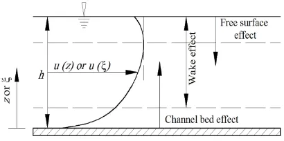
It is known that the velocity of turbulent flow in open channels is not uniformly distributed over the cross-section. This non-uniformity is caused by the presence of free surface and frictional resistance along the channel perimeter. The turbulent flow field in an open channel can be divided into three flow layers (Nezu and Nakagawa, 1993). These layers are defined as; wall shear layer (z <0.2 h), intermediate layer (0.2 h ≤ z ≤ 0.6 h) and free surface layer (0.6 h < z ≤ h), where
z is the distance from the solid boundary and h is the flow depth.
For the wall shear layer, which is also called the inner layer, the velocity distribution is found to follow the law of the wall (Chow, 1959). It is important to note that the velocity distribution in the wall shear layer (inner layer) does not depend on the free stream velocity or the maximum velocity (Umax). For the outer layer, which includes the free surface and intermediate layers, the flow velocity is dependent on the maximum velocity (Umax) as well as the bed shear stress, mass density of the fluid and flow depth, but it is independent of fluid viscosity, (Pope, 2000). Thus, the law of the velocity defect is found to be applicable in the outer layer.
The traditional laws, such as the law of the wall and velocity defect law, may fail to describe the velocity distribution in the outer region because they only consider the effect of the boundary walls and
neglect the free surface effect (Wang et al., 2001; Guo and Julien, 2003). The effect of the free surface on turbulence is particularly significant as it results in an anisotropy of turbulence, which in turn causes the generation of secondary flows. The secondary cells generated near the free surface is found to be responsible for the velocity-dip phenomenon, whereby the maximum velocity appears below the free surface (Nezu and Rodi, 1986). The velocity-dip phenomenon often occurs in narrow channels with an aspect ratio (Ar) being less than 5 (Nezu and Rodi, 1986, Yang
et al., 2004). The aspect ratio is defined as the ratio of the channel width to the water depth, (b/h). The velocity-dip may also occur in the central section of a wide channel whose aspect ratio is larger than 5, because of the variation of bed elevation along the lateral direction (Wang and Cheng, 2005).
Res. J. Appl. Sci. Eng. Technol., 16(1): 9-14, 2019
10
Fig. 1: Typical velocity profile of the narrow open channel flow
produce laws for velocity distribution that depend on parameters for characterizing the secondary flow, turbulence and boundary roughness. For uniform flows in narrow rectangular channels, Yang et al. (2004) derived an analytical model called Dip-Modified Logarithmic law (DML-law), including the velocity-dip phenomenon caused by the secondary flows. To simplify RANS equations, Yang et al. (2004) assume an empirical model for secondary flow term and use a parabolic distribution for eddy viscosity. The DML-law can be given as follows (Fig. 1):
𝑈 𝑢∗=
1 𝑘[𝑙𝑛 (
𝜉
𝜉𝑜) + 𝛼 𝑙𝑛(1 − 𝜉)] (1)
where,
u = Time-averaged velocity in the flow direction 𝑢∗ = Shear velocity
k = Von Karman constant
α = The dip-correction parameter which represents the secondary flow effect
𝜉 = Normalized distance relative to the flow depth h
(i.e., 𝜉 = 𝑧/ℎ) 𝜉𝑜 = Defined as (𝑧𝑜/ℎ)
𝑧𝑜 = The distance at which the velocity is hypothetically equal to zero
Although this law adequately reproduces the velocity profiles of many experimental flows, it is dedicated to smooth channels only (Wisam and Prasad, 2018). There is another analytical model for velocity distribution, which is called simple Dip-Modified Log-Wake law (DMLW-law) (Absi, 2009). In this model, instead of a parabolic distribution used in DML-law, the eddy viscosity (𝜈𝑡) is approximated in accordance
with the log-wake law given by Nezu and Rodi (1986). The DMLW-law can be given as follows:
𝑈 𝑢∗=
1 𝑘[𝑙𝑛 (
𝜉 𝜉𝑜) +
2Π 𝑘 sin
2(𝜋
2𝜉) + 𝛼 𝑙𝑛(1 − 𝜉)] (2)
where, Π is the known Coles parameter which expresses the strength of the wake (Coles, 1956). This parameter is suggested to interpret the disturbed flow and turbulent eddy mixing in the outer layer induced by
the side-walls of the channel or by gravity-pressure effects.
Many researchers (Guo and Julien, 2008; Absi, 2011; Lassabatere et al., 2012; Kundu, 2017) have then modified these two laws or proposed new laws by using the similar concept of the dip-modified laws. However, the DMLW-law differs from these modified models in that the former utilizes a number of parameters less than any other model and thus it would be simpler for the engineering application. In addition to that, the DMLW-law can be applicable to both smooth and rough flows. Therefore, only this law is considered in this study by discussing the model parameters (α and Π) and improving the methods that are used for estimating these parameters.
MATERIALS AND METHODS
As discussed in the preceding section, to apply the analytical model (DMLW-law), two parameters need first to be calculated. They are the wake strength parameter Π and the dip correction factor α. The present paper is aimed at proposing methods for a comprehensive estimation of the model parameters (Π, α) that would be applicable to both smooth and rough flows. To establish this objective, two sets of experiments that include rough and smooth flows were carried out. The details of these experiments are provided in the next subsection.
Experimental design: Two sets of experiments were conducted on rectangular channels that have two different beds in terms of the roughness. The experimental conditions for the experiments are given in Table 1. In the first set, which includes test cases (S6 to S20) in Table 1, the smooth stainless bed surface of the flume itself was used for establishing a hydraulically smooth flow condition. In the second group, which consists of experiments (R6 to R20), a single layer of grains (D84 = 8.0 mm) affixed to an aluminium plate was used to roughen the channel bed, as shown in Fig. 2. D84is the particle diameter so that 84% of the particles in the total grain-size distribution are smaller than D84. The equivalent sand roughness height (Ks) for the fully rough cases was estimated to be
the same order of magnitude as D84.
A Pitot tube with an inner diameter of 1.0 mm and with 4 holes (φ 0.75 mm) was used in the experiments to obtain vertical velocity profiles. The Pitot tube was connected to the low-range digital pressure transducer (Comark C9551/SIL, 0 to ±140 mbar), to measure the pressure difference (Δp) between the static and dynamic pressures. The point velocity can then be calculated from the pressure difference based on Bernoulli principle.
[image:3.612.83.288.82.184.2]Table 1: Experimental Conditions for all flow cases
Case Flow depth h (cm)
Aspect ratio Ar (---)
Flow rate Q (l/s)
Shear velocity
𝑢∗ (m/s)
Roughness condition Ks (mm)
S6 6.0 5.0 5.2 0.0159 ~ 0.15
S10 10.0 3.0 11.4 0.0183 ~ 0.15
S15 15.0 2.0 21.1 0.0197 ~ 0.15
S20 20.0 1.5 32.8 0.0211 ~ 0.15
R6 6.0 5.0 3.1 0.0153 8.0
R10 10.0 3.0 7.4 0.0187 8.0
R15 15.0 2.0 14.9 0.0221 8.0
R20 20.0 1.5 24.6 0.0239 8.0
1: The values of 𝑢∗ are the local shear velocity at the centre line of the channel; 2: The values of Ks for smooth cases are calculated based on the roughness manning coefficients (n)
(a) (b)
Fig. 2: Photos showing roughness conditions of rectangular channels; (a) Smooth flow and (b) Rough flow
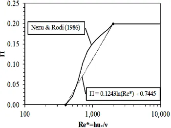
Fig. 3: The relationship between wake strength parameter (П) and 𝑅𝑒∗
bed slope of 0.0005. The flow depth (h) was changed with keeping the channel width (b) invariant to examine the effect the secondary flows on the velocity distributions. The adopted flow depths provide the range of aspect ratios (Ar = b/h) from 1.5 to 5, covering the same range as for narrow rectangular channels. In the narrow channels where Ar<5, strong secondary currents are developed and their effect on the primary flows is thought to be significant.
Calculation methods of model parameters: When analytical models based on the log wake are used, the values of the wake strength parameter (Π) and dip correction parameter (α) should be estimated carefully for accurate prediction of velocity. In open channel flows, the value of Π seems to be not universal where
many researchers suggested different values of Π, ranging from 0.08 (Cebeci and Smith, 1974) to 0.55 (Cardoso et al., 1989). Nezu and Rodi (1986) proved that the value of Π depends on the shear Reynolds number (𝑅𝑒∗= ℎ𝑢
∗/𝜈), as shown in Fig. 3. The figure indicates that at smaller values of 𝑅𝑒∗, Π increases rapidly with the Reynolds number but remains constant at Π = 0.2 beyond 𝑅𝑒∗ >2000. Based on this fact, the following equation, which expresses the dependency of the wake strength parameter Π on the roughness conditions of the flow, was suggested as a method for calculating Π in this study:
Π = 0.1243𝑙𝑛(𝑅𝑒∗) − 0.7445 for 𝑅𝑒∗≤ 2000 (3)
The value of dip correction parameter α can be determined from the distance of the maximum velocity from the bed as follows:
𝛼 = 1
𝜉𝑑𝑖𝑝− 1 (4)
where, 𝜉𝑑𝑖𝑝 is normalized distance of maximum velocity from the channel bed (= zmax/h). Experiments have shown that 𝜉𝑑𝑖𝑝 is mainly related to the lateral position (y /h) of the measured velocity profiles in the channel (Yang et al., 2004). Hence, the following empirical formula was proposed for the dip correction factor:
𝛼 = 𝐶1 𝑒𝑥𝑝(−𝐶2 𝑦
ℎ) (5)
Fig. 4: Relationship between α and y/h for smooth and rough flow cases
α = 1.3exp (-y/H)
α = 1.1exp (-y/H)
0.00 0.10 0.20 0.30 0.40 0.50 0.60 0.70
0.0 0.5 1.0 1.5 2.0 2.5 3.0
α
y/H
[image:4.612.100.270.214.340.2] [image:4.612.98.273.384.515.2] [image:4.612.333.540.549.707.2]Res. J. Appl. Sci. Eng. Technol., 16(1): 9-14, 2019
12 Equation (5) has been derived for smooth flow regime with C1= 1.3 and C2= 1.0 and y is equal to 0.5b at the centreline of the channel. The coefficient α was found not only to be dependent on the aspect ratio Ar, but also on the channel friction (Absi, 2009). When applying Eq. (5) to smooth flow cases considered here, the estimated values of α appear to be close to those calculated by Eq. (4) based on the measured distance of maximum velocity, as shown in Fig. 4. However, Fig. 4 also shows that the parameter C1 in Eq. (5) should be reduced from 1.3 to 1.1 to make the equation applicable for rough flow cases. Therefore, in this study, Eq. (5) was used to calculate α in smooth and rough flows, but with different values of C1 depending on the roughness conditions of the flow.
RESULTS AND DISCUSSION
The analytical Dip-Modified Log Wake Law (DMLW-law) given by Eq. (2) was used to obtain the velocity distribution for all flow cases considered in this study. The wake strength parameter (Π) and the dip correction parameter (α) were determined by using the proposed equations, i.e., Eq. (3) and (5). The values of α and Π calculated by the proposed methods are summarised in Table 2.
[image:5.612.315.541.229.358.2]To evaluate the impact of the wake and dip correction parameters, the predicted velocity profiles obtained by the Dip-Modified Log Wake law (DMLW-law) were compared with the experimental data of smooth and rough flow cases, as shown in Fig. 5 and 6. In the Figures, two values of Π were used, one was calculated from Eq. (3) that is proposed in this study and the other value is assumed to be a constant as 0.2. For the dip-correction parameters, their values were calculated by Eq. (5) with corresponding C1 coefficients for each flow case.
Table 2: Values of Π and α calculated by the proposed expressions Case No. 𝑅𝑒∗ Π from Eq. (3) α from Eq. (5)
S6 947.62 0.11 0.11
S10 1825.03 0.19 0.29 S15 2947.68 0.25 0.48 S20 4205.07 0.29 0.61
T6 885.72 0.10 0.10
T10 1801.23 0.19 0.27 T15 3089.01 0.25 0.44 T20 4456.81 0.30 0.57
R6 913.16 0.10 0.09
R10 1867.41 0.19 0.25 R15 3294.32 0.26 0.40 R20 4768.19 0.31 0.52
Re* is the shear Reynolds number, Π is the wake strength parameter and α is the velocity dip parameter.
(a) (b)
[image:5.612.108.505.387.707.2]
(c) (d)
(a) (b)
(c) (d)
Fig. 6: Comparison between analytical and experimental vertical distributions of U for rough flow cases; (a) R6 (h = 6.0 cm), (b) R10 (h = 10.0 cm, (c) R15 (h = 15.0 cm) and (d) R20 (h = 20.0 cm)
From Fig. 5, it can be noted that the value of Π plays an important role in obtaining accurate solutions for velocity distributions. For low flow cases (S6~S10), where the shear Reynolds number (𝑅𝑒∗) is less than 2000, the analytical profiles with Π calculated by Eq. (3) (solid lines) are more consistent with the experimental data than the profiles based on a constant value of Π, i.e., Π = 0.2 (dashed lines). In contrast, the results clearly show that the value of Π has no influence on the analytical solutions for high flow cases (S15 and S20), i.e., the cases with high shear Reynolds number (𝑅𝑒∗). For these flow cases, the velocity profiles obtained analytically do not agree well with the experimental data when Π calculated from the proposed expression are used. However, when Π remains constant at 0.20, the analytical profiles for velocity (dashed lines) are better and come closer to the experimental profiles. These results confirm the suggestion of depending the eddy viscosity and then Π on the shear Reynolds number 𝑅𝑒∗ up to a certain value (𝑅𝑒∗<2000). After this limit of 𝑅𝑒∗, Π takes a constant value at 0.2 even though 𝑅𝑒∗ increases. The application of the analytical model (DMLW-law) to smooth cases also shows that the dip-phenomena is reasonably predicted by using Eq. (5) with the standard value of the coefficient C1 (i.e., C1 = 1.3).
For comparison, the application of the analytical model to the rough flow cases has also been undertaken, as illustrated in Fig. 6. The results show that the analytical model can successfully predict velocity distributions for flows over rough surfaces. It is also clear from the figure that the DMLW-law is able to predict the maximum velocity and its position with an acceptable degree of accuracy. This means that the modification made on Eq. (5) by reducing the value of the coefficient C1 make the equation applicable to the rough flows and to the smooth flows as well. In addition, Fig. 6 shows the same influence of Π on the analytical results that was shown in smooth flow cases. The results indicate that using Π based on the proposed equation Eq. (3) gives good predicted velocity profiles in the cases of low flows (e.g., R6). But for high flows (e.g., R20), keeping Π constant at 0.20 leads to the best agreement between the analytical and experimental results. This clearly illustrates the effects of friction on estimating the value of Π and then on the results of the analytical solutions. The results in the present study confirm the findings obtained by Absi (2011) regarding the importance of the wake term for adequate prediction of the velocity distribution. However, according to Absi (2011), a greater value than that resulting from Eq. (3) was required to obtain accurately predicted velocity.
0.0 0.1 0.2 0.3 0.4 0.5 0.6 0.7 0.8 0.9 1.0
0.10 0.15 0.20 0.25
z/
h
U [m/s]
Experiment Analytical, Π = 0.10 Analytical, Π = 0.20
0.0 0.1 0.2 0.3 0.4 0.5 0.6 0.7 0.8 0.9 1.0
0.10 0.15 0.20 0.25 0.30
z/
h
U [m/s]
Experiment Analytical, Π = 0.19 Analytical, Π = 0.20
0.0 0.1 0.2 0.3 0.4 0.5 0.6 0.7 0.8 0.9 1.0
0.15 0.20 0.25 0.30 0.35 0.40
z/
h
U [m/s]
Experiment Analytical, Π = 0.26 Analytical, Π = 0.20
0.0 0.1 0.2 0.3 0.4 0.5 0.6 0.7 0.8 0.9 1.0
0.20 0.25 0.30 0.35 0.40 0.45
z/
h
U [m/s]
[image:6.612.114.502.85.409.2]Res. J. Appl. Sci. Eng. Technol., 16(1): 9-14, 2019
14
CONCLUSION
The analytical model called dip-modified log wake law (DMLW-law) has been used to predict the velocity distribution for smooth and rough flows. The DMLW-law includes the effects of the secondary flows and turbulence on the velocity distribution through using the wake and dip correction parameters (П and α). The impact of these two parameters on the velocity prediction was examined and proposed expressions have been proposed to estimate the values of the parameters for both smooth and rough flows. The main findings of the present study can be summarized as follows:
Both the wake and dip correction parameters have a significant impact on the accuracy of the velocity prediction for smooth and rough flow cases.
For smooth flows, the dip correction parameter (α) can be evaluated from the expression proposed by (Yang et al., 2004) and given in Eq. (5). However, for rough flows, this expression need to modify by changing the value of the coefficients C1 (from 1.3 to 1.1).
The results indicate that the method suggested in the present study to calculate the wake parameter (Π) can improve the application of the analytical model to smooth and rough flows.
REFERENCES
Absi, R., 2009. Analytical methods for velocity distribution and dip-phenomenon in narrow open-channel flows. Proceeding of the International
Workshop on Environmental Hydraulics
Theoretical, Experimental and Computational Solutions, pp: 127-129.
Absi, R., 2011. An ordinary differential equation for velocity distribution and dip-phenomenon in open channel flows. J. Hydraulic Res., 49(1): 82-89. Cardoso, A.H., W.H. Graf and G. Gust, 1989. Uniform
flow in a smooth open channel. J. Hydraulic Res., 27(5): 603-616.
Cebeci, T. and A.M. Smith, 1974. Analysis of Turbulent Boundary Layers, Academic Press, New York.
Chow, V.T., 1959. Open-channel hydraulics. McGraw-Hill, New York, pp: 680.
Coles, D., 1956. The law of the wake in the turbulent boundary layer. J. Fluid Mech., 1(2): 191-226. Guo, J. and P.Y. Julien, 2003. Modified log-wake law
for turbulent flow in smooth pipes. J. Hydraulic Res., 41(5): 493-501.
Guo, J. and P.Y. Julien, 2008. Application of modified log-wake law in open-channels. J. Appl. Fluid Mech., 1(2): 17-23.
Kundu, S., 2017. Prediction of velocity-dip-position over entire cross section of open channel flows using entropy theory. Environ. Earth Sci., 76(10): 363.
Lassabatere, L., J.H. Pu, H. Bonakdari, C. Joannis and F. Larrarte, 2012. Velocity distribution in open channel flows: Analytical approach for the outer region. J. Hydraulic Eng., 139(1): 37-43.
Nezu, I. and H. Nakagawa, 1993. Turbulence in Open-Channel Flows. IAHR Monograph Series, A.A. Balkema, Rotterdam.
Nezu, I. and W. Rodi, 1986. Open-channel flow measurements with a laser Doppler anemometer. J. Hydraulic Eng., 112(5): 335-355.
Pope, S.B., 2000. Turbulent Flows, Cambridge University Press, Cambridge.
Wang, X., Z.Y. Wang, M. Yu and D. Li, 2001. Velocity profile of sediment suspensions and comparison of log-law and wake-law. J. Hydraulic Res., 39(2): 211-217.
Wang, Z.Q. and N.S. Cheng, 2005. Secondary flows over artificial bed strips. Adv. Water Resour., 28(5): 441-450.
Wisam, A. and T.D. Prasad, 2018. Comparison of performance of simplified RANS formulations for velocity distributions against full 3D RANS model. Int. J. Hydraulic Eng., 7(2): 33-42.
Yang, S.Q., S.K. Tan and S.Y. Lim, 2004. Velocity distribution and dip phenomenon in smooth
uniform open channel flows. J. Hydraulic