www.hydrol-earth-syst-sci.net/19/3857/2015/ doi:10.5194/hess-19-3857-2015
© Author(s) 2015. CC Attribution 3.0 License.
Computation of vertically averaged velocities in irregular
sections of straight channels
E. Spada1, T. Tucciarelli1, M. Sinagra1, V. Sammartano2, and G. Corato3
1Dipartimento di Ingegneria Civile, Ambientale, Aerospaziale, dei Materiali (DICAM), Università degli studi di Palermo, Viale delle Scienze, 90128, Palermo, Italy
2Dipartimento di Ingegneria Civile, dell’Energia, dell’Ambiente e dei Materiali (DICEAM), Università Mediterranea di Reggio Calabria, Via Graziella, 89122, Reggio Calabria, Italy
3Centre de Recherche Public – Gabriel Lippmann, 41 rue du Brill, 4422 Belvaux, Luxembourg Correspondence to: E. Spada ([email protected])
Received: 9 February 2015 – Published in Hydrol. Earth Syst. Sci. Discuss.: 27 February 2015 Revised: 27 August 2015 – Accepted: 28 August 2015 – Published: 14 September 2015
Abstract. Two new methods for vertically averaged veloc-ity computation are presented, validated and compared with other available formulas. The first method derives from the well-known Huthoff algorithm, which is first shown to be de-pendent on the way the river cross section is discretized into several subsections. The second method assumes the verti-cally averaged longitudinal velocity to be a function only of the friction factor and of the so-called “local hydraulic ra-dius”, computed as the ratio between the integral of the ele-mentary areas around a given vertical and the integral of the elementary solid boundaries around the same vertical. Both integrals are weighted with a linear shape function equal to zero at a distance from the integration variable which is pro-portional to the water depth according to an empirical co-efficientβ. Both formulas are validated against (1) labora-tory experimental data, (2) discharge hydrographs measured in a real site, where the friction factor is estimated from an unsteady-state analysis of water levels recorded in two different river cross sections, and (3) the 3-D solution ob-tained using the commercial ANSYS CFX code, computing the steady-state uniform flow in a cross section of the Alzette River.
1 Introduction
Computation of vertically averaged velocities is the first step of two major calculations in 1-D shallow water modelling: (1) estimation of the discharge given the energy slope and
the water stage and (2) estimation of the bottom shear stress for computing the bedload in a given river section.
Many popular software tools, like MIKE11 (MIKE11, 2009), compute the dischargeQ, in each river section, as the sum of discharges computed in different subsections, assum-ing a sassum-ingle water stage for all of them. Similarly, HEC-RAS (HEC-RAS, 2010) calculates the conveyance of the cross section by the following form of Manning’s equation:
Q=KS1f/2, (1)
whereSf is the energy slope andKis the conveyance,
com-puted assuming the same hypothesis and solving each sub-section according to the traditional Manning equation.
The second option, called divided channel method (DCM) is to compute the total discharge as the sum of the discharges flowing in each convex part of the section (called subsec-tion), assuming a single water level for all parts (Chow, 1959; Shiono et al., 1999; Myers and Brennan, 1990). In this ap-proach, the wet perimeter of each subsection is restricted to the component of the original one pertaining to the subsec-tion, but the new components shared by each couple of sub-sections are neglected. This is equivalent to neglecting the shear stresses coming from the vortices with vertical axes (if subsections are divided by vertical lines) and considering additional resistance for higher velocities, which results in overestimation of discharge capacity (Lyness et al., 2001).
Knight and Hamed (1984) compared the accuracy of sev-eral subdivision methods for compound straight channels by including or excluding the vertical division line in the com-putation of the wetted perimeters of the main channel and the floodplains. However, their results show that conventional calculation methods result in larger errors. Wormleaton et al. (1982) and Wormleaton and Hadjipanos (1985) also dis-cussed, in the case of compound sections, the horizontal di-vision through the junction point between the main channel and the floodplains. Their studies show that these subdivi-sion methods cannot assess well the discharge in compound channels.
The interaction phenomenon in compound channels has also been extensively studied by many other researchers (e.g. Sellin, 1964; Knight and Demetriou, 1983; Stephenson and Kolovopoulos, 1990; Rhodes and Knight, 1994; Bous-mar and Zech, 1999; van Prooijen et al., 2005; Moreta and Martin-Vide, 2010). Their studies demonstrate that there is a large velocity difference between the main channel and the floodplain, especially at low relative depth, leading to a sig-nificant lateral momentum transfer. The studies by Knight and Hamed (1984) and Wormleaton et al. (1982) indicate that the vertical transfer of momentum between the upper and the lower main channels exists, causing significant horizontal shear able to dissipate a large part of the flow energy.
Furthermore, many authors have tried to quantify flow in-teraction among the subsections, at least in the case of com-pound but regular channels. To this end, turbulent stress was modelled through the Reynolds equations and coupled with the continuity equation (Shiono and Knight, 1991). This cou-pling leads to equations that can be analytically solved only under the assumption of negligible secondary flows. Ap-proximated solutions can also be obtained, although they are based on some empirical parameters. Shiono and Knight de-veloped the Shiono–Knight method (SKM) for prediction of lateral distribution of depth-averaged velocities and bound-ary shear stress in prismatic compound channels (Shiono and Knight, 1991; Knight and Shiono, 1996). The method can deal with all channel shapes that can be discretized into linear elements (Knight and Abril, 1996; Abril and Knight, 2004).
Other studies based on the Shiono and Knight method can be found in Liao and Knight (2007), Rameshwaran
and Shiono (2007), Tang and Knight (2008) and Omran and Knight (2010). Apart from SKM, some other methods for analysing the conveyance capacity of compound chan-nels have been proposed. For example, Ackers (1993) for-mulated the so-called empirical coherence method. Lam-bert and Sellin (1996) suggested a mixing length approach at the interface whereas, more recently, Cao et al. (2006) reformulated flow resistance through lateral integration us-ing a simple and rational function of depth-averaged veloc-ity. Bousmar and Zech (1999) considered the main chan-nel/floodplain momentum transfer proportional to the prod-uct of the velocity gradient at the interface times the mass discharge exchanged through this interface due to turbulence. This method, called EDM (exchange divided method), also requires a geometrical exchange correction factor and turbu-lent exchange model coefficient for evaluating discharge.
A simplified version of the EDM, called interactive di-vided channel method (IDCM), was proposed by Huthoff et al. (2008). In IDCM, lateral momentum is considered neg-ligible and turbulent stress at the interface is assumed to be proportional to the spanwise kinetic energy gradient through a dimensionless empirical parameterα. IDCM has the strong advantage of using only two parameters,αand the friction factor,f. Nevertheless, as shown in the next section,α de-pends on the way the original section is divided.
An alternative approach could be to simulate the flow structure in its complexity by using a 3-D code for compu-tational fluid dynamics (CFD). In these codes flow is rep-resented both in terms of transport motion (mean flow) and turbulence by solving the Reynolds-averaged Navier Stokes (RANS) equations (Wilcox, 2006) coupled with turbulence models. These models allow for closure of the mathemati-cal problem by adding a certain number of additional par-tial differenpar-tial transport equations equal to the order of the model. In the field of the simulation of industrial and environ-mental laws, second-order models (e.g.k–εandk–ωmodels) are widely used. Nonetheless, CFD codes need a mesh fine enough to solve the boundary layer (Wilcox, 2006), resulting in a computational cost that can be prohibitive even for rivers of few kilometres in length.
In this study, two new methods aimed at representing subsection interactions in a compound channel are pre-sented. The first method, named “integrated channel method” (INCM), derives from the Huthoff formula, which is shown to give results depending on the way the river cross sec-tion is discretized in subsecsec-tions. The same dynamic balance adopted by Huthoff is written in differential form, but its dif-fusive term is weighted according to aξ coefficient propor-tional to the local water depth.
orig-inal hydraulic radius is changed with a “local” one. This “lo-cal” hydraulic radius should take into account the effect of the surrounding section geometry, up to a maximum distance which is likely to be proportional to the local water depth, according to an empiricalβcoefficient. The method gives up the idea of solving the Reynolds equations, due to the uncer-tainty of its parameters, but relies on the solid grounds of the historical experience of the Manning equation.
The present paper is organized as follows: two of the most popular approaches adopted for computation of the vertically averaged velocities are explained in details along with the proposed INCM and LHRM methods. Theξ andβ parame-ters of, respectively, the INCM and LHRM methods are then calibrated from available laboratory experimental discharge data and a sensitivity analysis is carried out. The INCM and LHRM methods are finally validated according to three dif-ferent criteria. The first criterion is comparison with other series of the previous laboratory data not used for calibra-tion. The second criterion is comparison with discharge data measured in one section of the Alzette River basin (Luxem-bourg). Because the friction factor is not known a priori, the INCM and LHRM formulas are applied in the context of the indirect discharge estimation method, which simultaneously estimates the friction factor and the discharge hydrograph from the unsteady-state water level analysis of two water level hydrographs measured in two different river sections. The third validation criterion is comparison with the verti-cal velocity profiles obtained by the ANSYS CFX solver in a cross section of the Alzette River. In the conclusions, it is fi-nally shown that application of bedload formulas, carried out by integration of elementary solid fluxes computed as func-tion of the vertically averaged velocities, can lead to results that are strongly different from those obtained by using the simple mean velocity and water depth section values.
2 Divided channel method (DCM) and interactive divided channel method (IDCM)
In the DCM method the river section is divided into subsec-tions with uniform velocities and roughness (Chow, 1959). Division is made by vertical lines and no interaction between adjacent subsections is considered. Discharge is obtained by summing the contributions of each subsection, obtained by applying the Manning formula:
q=X
i qi=
X
i
R2i/3Ai ni
p
Sfi, (2)
whereqis the total discharge,Ai,Riandniare the area, the
hydraulic radius and the Manning roughness coefficient of each sub sectioniof a compound channel andSf is the
en-ergy slope, assumed constant across the river section. DCM is extensively applied in most of the commercial codes, two of them cited in the introduction.
In order to model the interaction between adjacent subsec-tions of a compound section, the Reynolds and the continuity equations can be coupled (Shiono and Knight, 1991) to get
ρ ∂ ∂y
H UvVd
=ρgH S0+ ∂ ∂y
H τxy
−τb
1+ 1 s2
1/2 , (3) whereρ is the water density, g is the gravity acceleration, yis the abscissa according to the lateral direction,UandV are, respectively, the velocity components along the flowx direction and the lateraly direction, H is the water depth, the subindexd marks the vertically averaged quantities and the bar the time average along the turbulence period,S0 is the bed slope,sis the section lateral slope, andτβis the bed
shear stress. Theτxy turbulent stress is given by the eddy
viscosity equation, i.e.
τxy=ρεxy ∂Ud
∂y , (4a)
εxy=λU∗H, (4b)
where the friction velocityU∗is set equal to
U∗=
f 8g
1/2
Ud, (5)
andf is the friction factor, depending on the bed material. The analytical solution of Eqs. (3)–(5) can be found only if the left-hand side of Eq. (3) is zero, which is equivalent to neglecting secondary flows. Other solutions can only be found by assuming a known0value for the lateral deriva-tive. Moreover,λ is another experimental factor depending on the section geometry. The result is that the solution of Eq. (3) strongly depends on the choice of two coefficients, λand0, which are additional unknowns with respect to the friction factorf.
In order to reduce to one the number of empirical param-eters (in addition tof) Huthoff et al. (2008) proposed the so-called interactive divided channel method (IDCM).
Integration of Eq. (3) over eachith subsection, neglecting the averaged flow lateral momentum, leads to
ρgAiS0=ρfiPiUi2+τi+1Hi+1+τiHi, (6)
where the left-hand side of Eq. (6) is the gravitational force per unit length, proportional to the density of waterρ, to the gravity accelerationg, to the cross-sectional areaAi, and to
the streamwise channel slopeS0. The terms on the right-hand side are the friction forces, proportional to the friction factor f and to the wet solid boundaryPi, and the turbulent lateral
momentum on the left and right sides, proportional to the turbulent stressτ and to the water depthH.
Turbulent stresses are modelled quite simply as
τi+1= 1 2ρα
whereα is a dimensionless interface coefficient,Ui2 is the square of the vertically averaged velocity and τi is the
tur-bulent stress along the plane between subsectioni−1 andi. If subsectioniis the first (or the last) one, velocityUi−1(or Ui+1) is set equal to zero.
Following a wall-resistance approach (Chow, 1959), the friction factorfiis computed as
fi = g n2i
Ri1/3
, (8)
whereni is the Manning’s roughness coefficient andRi(= Ai/Pi)is the hydraulic radius of subsectioni.
Equations (6) forms a system with an order equal to the number m of subsections, which is linear in the Ui2 un-knowns. The results are affected by the choice of theα co-efficient equal to 0.02, which is recommended by Huthoff et al. (2008), on the basis of lab experiments. Computation of the velocitiesUi makes it easy to estimate dischargeq.
IDCM has the main advantage of using only two param-eters, thef andαcoefficients. On the other hand, it can be easily shown thatα, although it is dimensionless, depends on the way the original section is divided. The reason is that the continuous form of Eq. (6) is given by
ρg
H S0− f U2 gcosθ
= ∂
∂y(τ H ) , (9)
whereθ is the bed slope in the lateral direction. Following the same approach as the IDCM, if we assume the turbulent stressτ to be proportional to both the velocity gradient in the lateral direction and to the velocity itself, we can write the right-hand side of Eq. (9) in the form
∂
∂y(τ H )= ∂ ∂y α H 2 ρU ∂U ∂yH , (10)
and Eq. (9) becomes ρ
gH S0− f U2 gcosθ
= ∂ ∂y H ∂ ∂y
αHρU2
. (11)
In Eq. (10)αHis no longer dimensionless, but is a length. To
get the same Huthoff formula from numerical discretization of Eq. (10), we should set
αH=0.021y, (12)
where 1y is the subsection width, i.e. the integration step size. This implies that the solution of Eq. (11), according to the Huthoff formula, depends on the way the equation is dis-cretized and the turbulence stress term on the right-hand side vanishes along with the integration step size.
3 The new methods
3.1 Integrated channel method (INCM)
INCM derives from the IDCM idea of evaluating the turbu-lent stresses as proportional to the gradient of the squared
averaged velocities, leading to Eqs. (7) and (11). Observe that the dimensionless coefficientα, in the stress computa-tion given by Eq. (7), can be written as the ratio between αH and the distance between verticalsi andi+1. For this
reason, coefficientαH can be thought of as a sort of
mix-ing length, related to the scale of the vortices with horizontal axes. INCM assumes the optimalαH to be proportional to
the local water depth, because water depth is at least an upper limit for this scale, and the following relationship is applied:
αH =ξ H, (13)
whereξ is an empirical coefficient to be further estimated. 3.2 Local hydraulic radius method (LHRM)
LHRM derives from the observation that, in the Manning equation, the average velocity is set equal to
V =R 2/3
n p
S0 (14)
and has a one-to-one relationship with the hydraulic radius. In this context the hydraulic radius has the meaning of a global parameter, measuring the interactions of the particles along all the section as the ratio between an area and a length. The inconvenience is that, according to Eq. (14), the verti-cally averaged velocities in points very far from each other remain linked anyway, because the infinitesimal area and the infinitesimal length around two verticals are summed to the numerator and to the denominator of the hydraulic radius in-dependently from the distance between the two verticals. To avoid this, LHRM computes the discharge as an integral of the vertically averaged velocities in the following form:
q= L
Z
0
h (y) U (y)dy, (15)
whereUis set equal to
U=< 2/3 1 n
p
S0, (16)
and<1is defined as local hydraulic radius, computed as
<1(y)=
Rb
ah (s) N (y, s)ds
Rb aN (y, s)
√
ds2+dz2, (17a)
a=max(0, y−βh) , (17b)
b=min(L, y+βh) , (17c)
wherezis the topographic elevation (function ofs),β is an empirical coefficient andLis the section’s top width. More-overN (y, s)is a shape function where
N (y, s)=
−[y−βh(y)]−s
βh(y) if a < s < y,
[y−βh(y)]−s
βh(y) if b > s > y,
0 otherwise.
Equation (18) shows how the influence of the section geom-etry, far from the abscissay, continuously decreases up to a maximum distance, which is proportional to the water depth according to an empirical positive coefficient β. After nu-merical discretization, Eqs. (15)–(17) can be solved to get the unknownq, as well as the vertically averaged velocities in each subsection. Ifβ is close to zero and the size of each subsection is common for both formulas, LHRM is equiva-lent to DCM; if β is very large, LHRM is equivalent to the traditional Manning formula. In the following,βis calibrated using experimental data available in the literature. A sensi-tivity analysis is also carried out to show that the estimated discharge is only weakly dependent on the choice of theβ coefficient, far from its possible extreme values.
3.3 Evaluation of theξ andβparameters by means of lab experimental data
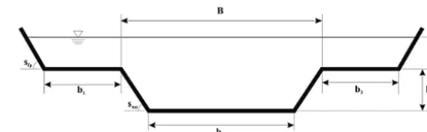
INCM and LHRM parameters were calibrated by using data selected from six series of experiments run at the large-scale Flood Channel Facility (FCF) of HR Wallingford (UK) (Knight and Sellin, 1987; Shiono and Knight, 1991; Ackers, 1993), as well as from four series of experiments run in the small-scale experimental apparatus of the Civil Engineering Department at the University of Birmingham (Knight and Demetriou, 1983). The FCF series were named F1, F2, F3, F6, F8 and F10; the Knight and Demetriou series were named K1, K2, K3 and K4. Series F1, F2, and F3 covered differ-ent floodplain widths, while series F2, F8, and F10 kept the floodplain widths constant but covered different main chan-nel side slopes. Series F2 and F6 provided a comparison be-tween the symmetric case of two floodplains and the asym-metric case of a single floodplain. All the experiments of Knight and Demetriou (1983) were run with a vertical main channel wall but with differentB/bratios. The series K1 has B/b=1 and its section is simply rectangular. TheB/bratio, for Knight’s experimental apparatus, was varied by adding an adjustable side wall to each of the floodplains either in pairs or singly to obtain a symmetrical or asymmetrical cross sec-tion. The geometric and hydraulic parameters are shown in Table 1; all notations of the parameters can be found in Fig. 1 andS0is the bed slope. The subscripts mc and fp of the side slope refer to the main channel and floodplain, respectively. Perspex was used for both main flume and floodplains in all tests. The related Manning roughness is 0.01 m−1/3s.
The experiments were run with several channel configura-tions, differing mainly for floodplain geometry (widths and side slopes) and main channel side slopes (see Table 1). The K series were characterized by vertical main channel walls. More information concerning the experimental setup can be found in Table 1 (Knight and Demetriou, 1983; Knight and Sellin, 1987; Shiono and Knight, 1991).
[image:5.612.309.545.65.138.2]Four series, named F1, F2, F3 and F6, were selected for calibration of theβcoefficient using the Nash–Sutcliffe (NS)
[image:5.612.312.541.204.333.2]Figure 1. Geometric parameters of a compound channel.
Table 1. Geometric and hydraulic laboratory parameters of the ex-periment series.
Series S0 h B b4 b1 b3 sfp smc
[%0] [m] [m] [m] [m] [m] [–] [–] F1
1.027 0.15 1.8 1.5
4.1 4.100 0 1
F2 2.25 2.250 1 1
F3 0.75 0.750 1 1
F6 2.25 0 1 1
F8 2.25 2.250 1 0
F10 2.25 2.250 1 2
K1
0.966 0.08 0.15 0.152
0.229 0.229
0 0
K2 0.152 0.152
K3 0.076 0.076
K4 – –
index of the measured and the computed flow rates as a mea-sure of the model’s performance (Nash and Sutcliffe, 1970). The remaining three series, named F2, F8 and F10, plus four series from Knight and Demetriou (1983), named K1, K2, K3 and K4, were used for validation (no.) 1, as reported in the next section. NS is given by
NS=
1−
P j=1,2
P i=1,NJ
P K=1,MNJ
qi,j,kobs −qi,j,ksim2
P j=1,2
P i=1,NJ
P K=1,MNJ
qi,j,kobs −qi,j,kobs 2
, (19) whereNjis the number of series,MNj is the number of tests
for each series,qi,j,ksim and qi,j,kobs are, respectively, the com-puted and the observed discharge (j=1 for the FCF series andj=2 for the Knight series;iis the series index; andK is the water depth index).qi,j,kobs is the average value of the measured discharges.
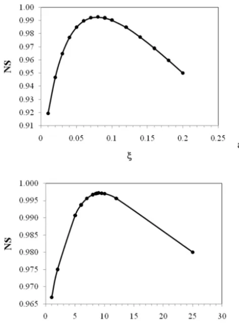
Bothξ andβ parameters were calibrated by maximizing the NS index, computed using all the data of the four series used for calibration. See the NS versus ξ andβ curves in Fig. 2a and b.
Calibration provides optimalξ andβ coefficients, respec-tively, equal to 0.08 and 9. The authors will show in the next sensitivity analysis that even a one-digit approximation of the ξandβcoefficients provides a stable discharge estimation. 3.4 Sensitivity analysis
Figure 2. NS versusξandβcurves, respectively, for INCM (a) and LHRM (b) methods.
normalized in the following form:
Is=
1 qINCM
1q
1ξ, (20)
Ls=
1 qLHRM
1q
1β, (21)
where1qis the difference between the discharges computed using two differentβ andξ values. The assumed perturba-tions “1β” and “1ξ” are, respectively, 1β=0.001β and 1ξ =0.001ξ.
The results of this analysis are shown in Table 2 for the F2 series, whereH is the water depth andQmeasthe corre-sponding measured discharge.
They show very low sensitivity of both the INCM and LHRM results, such that a one-digit approximation of both model parameters (ξ andβ) should guarantee a computed discharge variability of less than 2 %.
The results of the sensitivity analysis, carried out for se-ries K4 and shown in Table 2, are similar to the previous ones computed for F2 series.
Table 2. SensitivitiesIs andLs computed in the F2 and K4 series for the optimal parameter values.
H Qmeas Is Ls
[m] [m3s−1]
F2
series
0.156 0.212 0.2209 0.2402
0.169 0.248 0.1817 0.2194
0.178 0.282 0.1651 0.2044
0.187 0.324 0.1506 0.1777
0.198 0.383 0.1441 0.1584
0.214 0.480 0.1305 0.1336
0.249 0.763 0.1267 0.1320
K4
series
0.085 0.005 0.3248 0.3282
0.096 0.008 0.2052 0.2250
0.102 0.009 0.1600 0.1709
0.114 0.014 0.1354 0.1372
0.127 0.018 0.1174 0.1208
0.154 0.029 0.0851 0.0866
4 Validation criterion
4.1 Validation no. 1 – comparison with laboratory experimental data
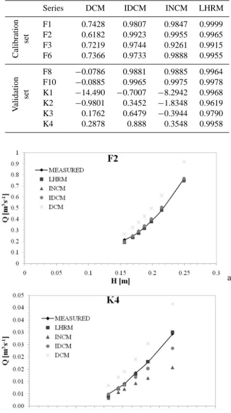
A first validation of the two methods was carried out by us-ing the calibrated parameter values, the same Nash–Sutcliffe performance measure and all the available experimental se-ries. The results were also compared with results of DCM and IDCM methods, the latter applied using the suggested α=0.02 value and five subsections, each one corresponding to a different bottom slope in the lateralydirection. The NS index for all data series is shown in Table 3.
The DCM results are always worse and are particularly bad for all the K series. The results of both the IDCM and INCM methods are very good for the two F series not used for calibration but are both poor for the K series. The LHRM method was always the best and also performed very well in the K series. The reason is probably that the K series tests have very low discharges and the constantα=0.02, the co-efficient adopted in the IDCM method, does not fit the size of the subsections, and Eq. (13) is not a good approximation of the mixing lengthαH in Eq. (12) for low values of the
wa-ter depth. In Fig. 3a and b the NS curves obtained by using DCM, IDCM, INCM and LHRM, for series F2 and K4, are shown.
4.2 Validation no. 2 – comparison with field data Although rating curves are available in different river sites around the world, field validation of the uniform flow formu-las is not easy for at least two reasons.
[image:6.612.343.514.96.280.2]Table 3. Nash–Sutcliffe efficiency for all (calibration and valida-tion) experimental series.
Series DCM IDCM INCM LHRM
Calibration
set
F1 0.7428 0.9807 0.9847 0.9999 F2 0.6182 0.9923 0.9955 0.9965 F3 0.7219 0.9744 0.9261 0.9915 F6 0.7366 0.9733 0.9888 0.9955
V
alidation set
F8 −0.0786 0.9881 0.9885 0.9964 F10 −0.0885 0.9965 0.9975 0.9978 K1 −14.490 −0.7007 −8.2942 0.9968 K2 −0.9801 0.3452 −1.8348 0.9619 K3 0.1762 0.6479 −0.3944 0.9790 K4 0.2878 0.888 0.3548 0.9958
Figure 3. Estimated discharge values against HR Wallingford FCF measures for F2 (a) and K4 (b) series.
the Manning coefficient to be compared with the actu-ally measured discharges.
2. River bed roughness does change, along with the Man-ning coefficient from one water stage to another (it usu-ally increases along with the water level).
A possible way to circumvent the problem is to apply the compared methods in the context of a calibration problem, where both the average Manning coefficient and the dis-charge hydrograph are computed from the known level hy-drographs measured in two different river cross sections (Pe-rumal et al., 2007; Aricò et al., 2009). The authors solved the
diffusive wave simulation problem using one known level hy-drograph as the upstream boundary condition and the second one as the benchmark downstream hydrograph for the Man-ning coefficient calibration.
It is well known in the parameter estimation theory (Aster et al., 2012) that the uncertainty of the estimated parameters (in our case the roughness coefficient) grows quickly with the number of parameters, even if the matching between the measured and the estimated model variables (in our case the water stages in the downstream section) improves. The use of only one single parameter over all the computational domain is motivated by the need of getting a robust estimation of the Manning coefficient and of the corresponding discharge hydrograph.
Although the accuracy of the results is restricted by sev-eral modelling assumptions, a positive indication about the robustness of the simulation model (and the embedded rela-tionship between the water depth and the uniform flow dis-charge) is given by (1) the match between the computed and the measured discharges in the upstream section, and (2) the compatibility of the estimated average Manning coefficient with the site environment.
The area of interest is located in the Alzette River basin (Grand Duchy of Luxembourg) between the gauged sections of Pfaffenthal and Lintgen (Fig. 4). The river reach length is about 19 km, with a mean channel width of∼30 m and an av-erage depth of∼4 m. The river meanders in a relatively large and flat plain about 300 m, with a mean slope of∼0.08 %.
The methodology was applied to a river reach 13 km long, between two instrumented sections, Pfaffenthal (upstream section) and Hunsdorf (downstream section), in order to have no significant lateral inflow between the two sections.
Events of January 2003, January 2007 and January 2011 were analysed. For these events, stage records and reliable rating curves are available at the two gauging stations of Pfaf-fenthal and Hunsdorf. The main hydraulic characteristics of these events, namely duration (1t), peak water depth (Hpeak) and peak discharge (qpeak), are shown in Table 4.
In this area a topographical survey of 125 river cross sec-tions was available. The hydrometric data were recorded ev-ery 15 min. The performances of the discharge estimation procedures were compared by means of the Nash–Sutcliffe criterion.
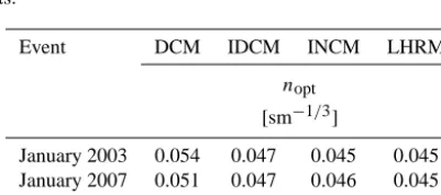
The results of the INCM and LHRM methods were also compared with those of the DCM and IDCM methods, the latter applied by usingα=0.02 and an average subsection width equal to 7 m. The computed average Manning coeffi-cientsnopt, reported in Table 5, are all consistent with the site environment, although they attain very large values, accord-ing to DCM an IDCM, in the 2011 event.
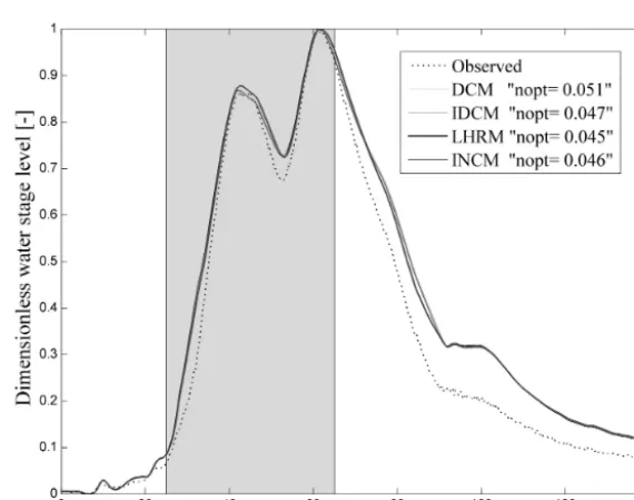
The estimated and observed dimensionless water stages in the Hunsdorf gauged site for the 2003, 2007 and 2011 events are shown in Figs. 5–7.
Figure 4. The Alzette study area.
Table 4. Main characteristics of the flood events at the Pfaffenthal and Hunsdorf gauged sites.
Event 1t Pfaffenthal Hunsdorf [h]
Hpeak qpeak Hpeak Qpeak
[m] [m3s−1] [m] [m3s−1] January 2003 380 3.42 70.98 4.52 67.80 January 2007 140 2.90 53.68 4.06 57.17 January 2011 336 3.81 84.85 4.84 75.10
Table 5. Optimum roughness coefficient,nopt, for the three flood
events.
Event DCM IDCM INCM LHRM
nopt
[sm−1/3]
January 2003 0.054 0.047 0.045 0.045
January 2007 0.051 0.047 0.046 0.045
January 2011 0.070 0.070 0.057 0.055
The falling limb is not included, since it has a lower slope and is less sensitive to the Manning coefficient value.
A good match between recorded and simulated discharge hydrographs can be observed (Figs. 8–10) in the upstream gauged site for each event.
For all investigated events the Nash–Sutcliffe efficiency NSqis greater than 0.90, as shown in Table 6.
[image:8.612.327.528.95.181.2]The error obtained between measured and computed dis-charges, with all methods, is of the same order of magnitude as the discharge measurement error. Moreover, this measure-ment error is well known to be much larger around the peak flow, where the estimation error has a larger impact on the NS
Table 6. Nash–Sutcliffe efficiency of estimated discharge hydro-graphs for the analysed flood events.
Event DCM IDCM INCM LHRM
NSq [–]
January 2003 0.977 0.987 0.991 0.989
January 2007 0.983 0.988 0.989 0.992
January 2011 0.898 0.899 0.927 0.930
coefficient. The NS coefficients computed with the LHRM and INCM methods are anyway a little better than the other two.
4.3 Validation no. 3 – comparison with results of 3-D ANSYS CFX solver
The vertically averaged velocities computed using DCM, IDCM, INCM and LHRM were compared with the results of the well-known ANSYS 3-D code, named CFX, which solves the RANS equations, applied to a prismatic reach with the irregular cross section measured at the Hunsdorf gauged section of the Alzette River. The length of the reach is about 4 times the top width of the section.
In the homogeneous multiphase model adopted by CFX, water and air are assumed to share the same dynamic fields of pressure, velocity and turbulence and water is assumed to be incompressible. CFX solves the conservation of mass and momentum equations, coupled with the air pressure– density relationship and the global continuity equation in each node. We denote α1,ρ1, µ1 and U1, respectively, as the volume fraction, the density, the viscosity and the time-averaged value of the velocity vector for phasel(l=w (wa-ter), a (air)), i.e.
ρ= X
l=w,a
α1ρ1, (22a)
µ= X
l=w,a
α1µ1, (22b)
whereρandµare the density and the viscosity of the “aver-aged” phase. The air density is assumed to be a function of the pressurep, according to the state equation:
ρa=ρa,0eγ (p−p0), (22c)
where the subindex 0 marks the reference state values andγ is the air compressibility coefficient.
The governing equations are the following: (1) the mass conservation equation, (2) the Reynolds-averaged continuity equation of each phase and (3) the Reynolds-averaged mo-mentum equations. Mass conservation implies
X
l = w, a
[image:8.612.66.267.464.553.2]Figure 5. Observed and simulated stage hydrographs at the Hunsdorf gauged site in the event of January 2003.
Figure 6. Observed and simulated stage hydrographs at the Hunsdorf gauged site in the event of January 2007.
The Reynolds-averaged continuity equation of each phase l can be written as
∂ρ1
∂t + ∇ ·(ρ1U)=S1, (24)
whereS1is an external source term. The momentum equation instead refers to the “averaged” phase and is written as
∂ (ρU)
∂t + ∇ ·(ρU⊗U)− ∇ ·
µeff
∇U+(∇U)T
+ ∇p0=SM, (25)
where⊗is the dyadic symbol,SMis the momentum of the external source termS, andµeffis the effective viscosity ac-counting for turbulence and defined as
[image:9.612.154.439.329.554.2]Figure 7. Observed and simulated stage hydrographs at the Hunsdorf gauged site in the event of January 2011.
Figure 8. Observed and simulated discharge hydrographs at the Pfaffenthal gauged site in the event of January 2003.
whereµt is the turbulence viscosity andp0is the modified pressure, equal to
p0=p+2
3ρk+ 2
3µeff∇ ·U, (27)
wherekis the turbulence kinetic energy, defined as the vari-ance of the velocity fluctuations andpis the pressure. Both phases share the same pressurepand the same velocity U.
To close the set of six scalar equations (Eqs. 23–25), we finally apply the k–εturbulence model implemented in the
CFX solver. The implemented turbulence model is a two equation model, including two extra transport equations to represent the turbulent properties of the flow.
[image:10.612.156.440.328.554.2]wall-Figure 9. Observed and simulated discharge hydrographs at the Pfaffenthal gauged site in the event of January 2007.
Figure 10. Observed and simulated discharge hydrographs at the Pfaffenthal gauged site in the event of January 2011.
bounded and internal flows, the model gives good results but only in cases where the mean pressure gradients are small.
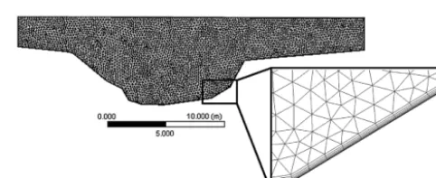
The computational domain was divided using both tetra-hedral and prismatic elements (Fig. 11). The prismatic ele-ments were used to discretize the computational domain in the near-wall region over the river bottom and the boundary surfaces, where a boundary layer is present, while the tetra-hedral elements were used to discretize the remaining do-main. The number of elements and nodes in the mesh used
for the specific case are of the order of, respectively, 4×10⁶ and 20×106.
A section of the mesh is shown in Fig. 12. The quality of the mesh was verified by using a pre-processing procedure by ANSYS®ICEM CFD™(Ansys Inc., 2006).
[image:11.612.157.440.328.550.2]Table 7. Boundary conditions assigned in the CFX simulation.
Geometry face Boundary condition
Inlet All velocity components
Outlet Velocity direction and hydrostatic pressure distribution
Side walls Opening
Top Opening
[image:12.612.45.289.121.349.2]Bottom No-slip wall condition, with roughness given by equivalent granular sized50
Figure 11. Computational domain of the reach of the Alzette River.
In the outlet section the hydrostatic distribution is given, the velocity is assumed to be still normal to the section and its norm is left unknown. All boundary conditions are reported in Table 7.
The opening condition means that that velocity direction is set normal to the surface, but its norm is left unknown and a negative (entering) flux of both air and water is allowed. Along open boundaries the water volume fraction is set equal to zero. The solution of the problem converges towards two extremes: nodes with zero water fraction, above the water level, and nodes with zero air fraction, below the water level. On the bottom boundary, between the nodes with zero ve-locity and the turbulent flow, a boundary layer exists that would require the modelling of microscale irregularities. CFX allows using, inside the boundary layer, a velocity log-arithmic law, according to an equivalent granular size. The relationship between the granular size and Manning’s coeffi-cient, according to Yen (1992), is given by
d50= n
0.0474 6
, (28)
whered50is the average granular size to be given as the input in the CFX code.
[image:12.612.307.548.187.285.2]Observe that the assumption of known and constant ve-locity directions in the inlet and outlet sections is a simpli-fication of reality. A more appropriate boundary condition at the outlet section, not available in the CFX code, would have been given by zero velocity and turbulence gradients
[image:12.612.308.549.323.378.2]Figure 12. A mesh section along the inlet surface.
Figure 13. Hunsdorf river cross section: subsections used to com-pute the vertically averaged velocities.
(Rameshwaran et al., 2013). For this reason, a better recon-struction of the velocity field can be found in an intermediate section, where secondary currents with velocity components normal to the mean flow direction can be easily detected (Pe-ters and Goldberg, 1989; Richardson and Thorne, 1998). See in Fig. 13 how the intermediate section was divided to com-pute the vertically averaged velocities in each segment sec-tion. These 3-D numerical simulations confirm that the mo-mentum0, proportional to the derivative of the average tan-gent velocities and equivalent to the left-hand side of Eq. (2), cannot be set equal to zero if a rigorous reconstruction of the velocity field is sought after.
To compute the uniform flow discharge, for a given outlet section, the CFX code is run iteratively, each time with a dif-ferent average longitudinal velocity in the inlet section, until the same water depth as in the outlet section is attained in the inlet section for steady-state conditions. Using the velocity distribution computed in the middle section along the steady-state computation as upstream boundary condition, transient analysis is carried on until pressure and velocity oscillations become periodic.
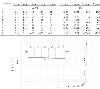
compo-Table 8. Simulated mean velocities in each segment section using 1-D hydraulic models with DCM, IDCM, INCM, LHRM and CFX, and the corresponding differences.
Subsection uCFX uDCM uIDCM uINCM uLHRM 1uDCM 1uIDCM 1uINCM 1uLHRM
[ms−1] [%]
1 1.33 1.58 1.47 1.23 1.12 18.79 10.52 −7.52 −15.78
2 1.37 1.42 1.4 1.36 1.38 3.65 2.19 −0.73 0.73
3 1.38 1.53 1.48 1.38 1.4 10.87 7.25 0 1.45
4 1.47 1.64 1.6 1.56 1.57 11.56 8.84 6.13 6.80
5 1.53 1.94 1.8 1.59 1.61 26.79 17.65 3.92 5.23
6 1.57 2.01 1.81 1.6 1.68 28.02 15.29 1.91 7.00
7 1.46 1.66 1.65 1.49 1.5 13.69 13.01 2.05 2.74
8 1.42 1.48 1.46 1.44 1.43 4.22 2.82 1.40 0.70
9 0.88 0.91 0.90 0.70 0.69 3.40 2.27 −20.45 −21.59
Figure 14. Streamwise vertical profile along the longitudinal axis of the mean channel.
nents for 10 verticals equally spaced along the longitudinal axis of the main channel. See in Fig. 14 the plot of four of them and their locations. The streamwise velocity evolves longitudinally and becomes almost completely self-similar starting from the vertical line in the middle section.
The stability of the results was finally checked against the variation of the length of the simulated channel. The dimen-sionless sensitivity of the discharge with respect to the chan-nel length is equal to 0.2 %.
See in Table 8 the comparison between the vertically av-eraged state velocities, computed through the DCM, IDCM, INCM and LHRM formulas (uDCM,uIDCM,uINCM,uLHRM) and through the CFX code (uCFX). Table 8 also shows the relative difference,1u, evaluated as
1u=u−uCFX uCFX
·100. (29)
[image:13.612.88.512.92.470.2]5 Conclusions
Two new methods computing the vertically averaged veloc-ities along irregular sections have been presented. The first method, named INCM, develops from the original IDCM method and it is shown to perform better than the previous one, with the exception of lab tests with very small discharge values. The second one, named LHRM, has empirical bases and gives up the ambition of estimating turbulent stresses but has the following important advantages.
1. It relies on the use of only two parameters: the friction factorf (or the corresponding Manning coefficientn) and a second parameter β, which on the basis of the available laboratory data, was estimated to be equal to 9.
2. Theβcoefficient has a simple and clear physical mean-ing: the correlation distance, measured in water depth units, of the vertically averaged velocities between two different verticals of the river cross section.
3. The sensitivity of the results with respect to the model β parameter was shown to be very low, and a one-digit approximation is sufficient to get a discharge variabil-ity of less than 2 %. A fully positive validation of the method was carried out using lab experimental data as well as field discharge and roughness data obtained by using the unsteady-state level analysis proposed by Ar-icò et al. (2009) and applied to the Alzette River in the Grand Duchy of Luxembourg.
4. Comparison between the results of the CFX 3-D turbu-lence model and the LHRM model shows a very good match between the two computed total discharges, al-though the vertically averaged velocities computed by the two models are quite different near to the banks of the river.
Moreover, the estimation of the velocity profiles in each of the considered subsections could be used in order to eval-uate the vertical average velocity and thus the shear stresses at the boundary of the whole cross section. In fact, it is well known that bedload transport is directly related to the bed shear stress and that this is proportional in each point of the section to the second power of the vertically averaged veloc-ity, according to Darcy and Weisbach (Ferguson, 2007): τ0=ρU2
f
8. (30)
All the bedload formulas available in the literature compute the solid flux per unit width. For example, the popular Schok-litsch formula (Gyr and Hoyer, 2006) is
qs=
2.5 ρs/ρ
S32(q−qc) , (31)
whereqandqsare, respectively, the liquid and the solid
Appendix A
Table A1. Notations.
Ai area of each subsection “i” of a compound channel
B top width of compound channel
b main channel width at bottom
f friction factor
g gravity acceleration
H total depth of a compound channel
nmc,nfp Manning’s roughness coefficients for the main channel and floodplain, respectively Pi wetted perimeter of each subsection “i” of a compound channel
Qmeas measured discharge
Ri hydraulic radius of each subsection “i” of a compound channel
S0 longitudinal channel bed slope
Sf energy slope
τ turbulent stress
ε turbulent dissipation
ρ fluid density
µ fluid viscosity
α IDCM interface coefficient
β LHRM coefficient
Acknowledgements. The authors wish to express their gratitude
to the Administration de la gestion de l’eau of the Grand-Duché de Luxembourg and the Centre de Recherche Public Gabriel Lippmann for providing hydrometric and topographical data of the Alzette River.
Edited by: R. Moussa
References
Abril, J. B. and Knight, D. W.: Stage-discharge prediction for rivers in flood applying a depth-averaged model, J. Hydraul. Res., 42, 616–629, 2004.
Ackers, P.: Flow formulae for straight two-stage channels, J. Hy-draul. Res., 31, 509–531, 1993.
Ansys Inc.: ANSYS CFX Reference guide, Canonsburg, Pennsyl-vania, USA, 2006.
Aricò, C., Nasello, C., and Tucciarelli, T.: Using unsteady water level data to estimate channel roughness and discharge hydro-graph, Adv. Water Resour., 32, 1223–1240, 2009.
Aster, C., Borchers, B., and Clifford, H.: Parameter Estimation and Inverse Problems, Elsevier, Academic Press, USA, 2012. Bousmar, D. and Zech, Y.: Momentum transfer for practical flow
computation in compound channels, J. Hydraul. Eng., 125, 696– 706, 1999.
Cao, Z., Meng, J., Pender, G., and Wallis, S.: Flow resistance and momentum flux in compound open channels, J. Hydraul. Eng., 132, 1272–1282, 2006.
Chow, V. T.: Open Channel Hydraulics, McGraw-Hill, New York, 1959.
Ferguson, R.: Flow resistance equations for gravel and boulder-bed streams, Water Resour. Res., 43, W05427, doi:10.1029/2006WR005422, 2007.
Gyr, A. and Hoyer, K.: Sediment Transport A geophysical Phe-nomenon, Springer, A. A Dordrecht, The Netherlands, 30–31, 2006.
HEC-RAS, River Analysis System, Hydraulic Reference Manual, US Army Corps of Engineers, Hydrologic Engineering Center, Davis, CA, 411 pp., 2010.
Herschel, C.: On the origin of the Chezy formula, Journal Associa-tion of Engineering Societies, 18, 363–368, 1897.
Huthoff, F., Roos, P. C., Augustijn, D. C. M., and Hulscher, S. J. M. H.: Interacting divided channel method for compound channel flow, J. Hydraul. Eng., 134, 1158–1165, 2008.
Jones, W. P. and Launder, B. E.: The prediction of laminarization with a two-equation model of turbulence, Int. J. Heat Mass Tran., 15, 301–314, 1972.
Knight, D. W. and Abril, B.: Refined calibration of a depth averaged model for turbulent flow in a compound channel, P. I. Civil Eng.-Water, 118, 151–159, 1996.
Knight, D. W. and Demetriou, J. D.: Flood plain and main channel flow interaction, J. Hydraul. Eng., 109, 1073–1092, 1983. Knight, D. W. and Hamed, M. E.: Boundary shear in symmetrical
compound channels, J. Hydraul. Eng., 110, 1412–1430, 1984. Knight, D. W. and Sellin, R. H. J.: The SERC flood channel facility,
J. Inst. Water Env. Man., 1, 198–204, 1987.
Knight, D. W. and Shiono, K.: River channel and floodplain hy-draulics, in: Floodplain Processes, edited by: Anderson, M. G.,
Walling, D. E., and Bates, P. D., Wiley, New York, Chapter 5, 139–181, 1996.
Lambert, M. F. and Sellin, R. H. J.: Discharge prediction in straight compound channels using the mixing length concept, J. Hydraul. Res., 34, 381–394, 1996.
Launder, B. E. and Sharma, B. I.: Application of the energy dissi-pation model of turbulence to the calculation of flow near a spin-ning disc, Lett. Heat Mass Trans., 1, 131–138, 1974.
Liao, H. and Knight, D. W.: Analytic stage-discharge formulas for flow in straight prismatic channels, J. Hydraul. Eng., 133, 1111– 1122, 2007.
Lyness, J. F., Myers, W. R. C., Cassells, J. B. C., and O’Sullivan, J. J.: The influence of planform on flow resistance in mobile bed compound channels, P. I. Civil Eng.-Water, 148, 5–14, 2001. MIKE11: A Modelling System for Rivers and Channels, Reference
Manual, DHI, Denmark, 524 pp., 2009.
Moreta, P. J. M. and Martin-Vide, J. P.: Apparent friction coefficient in straight compound channels, J. Hydraul. Res., 48, 169–177, 2010.
Myers, W. R. C. and Brennan, E. K.: Flow resistance in compound channels, J. Hydraul. Res., 28, 141–155, 1990.
Nash, J. E. and Sutcliffe, J. V.: River flow forecasting through con-ceptual models, Part I - A discussion of principles, J. Hydrol., 10, 282–290, 1970.
Omran, M. and Knight, D. W.: Modelling secondary cells and sedi-ment transport in rectangular channels, J. Hydraul. Res., 48, 205– 212, 2010.
Peters, J. J. and Goldberg, A.: Flow data in large alluvial channels, in: Computational Modeling and Experimental methods in Hy-draulics, edited by: Maksimovic, C. and Radojkovic, M., Else-vier, London, 77–86, 1989.
Perumal, M., Moramarco, T., Sahoo, B., and Barbetta, S.: A methodology for discharge estimation and rating curve devel-opment at ungauged river sites, Water Resour. Res., 43, W02412, doi:10.1029/2005WR004609, 2007.
Rameshwaran, P. and Shiono, K.: Quasi two-dimensional model for straight overbank flows through emergent vegetation on flood-plains, J. Hydraul. Res., 45, 302–315, 2007.
Rameshwaran, P., Naden, P., Wilson, C., Malki, R., Shukla, D., and Shiono, K.: Inter-comparison and validation of computational fluid dynamics codes in two-stage meander-ing channel flows, Appl. Math. Model., 37, 8652–8672, doi:10.1016/j.apm.2013.07.016, 2013.
Rhodes, D. G. and Knight, D. W.: Velocity and boundary shear in a wide compound duct, J. Hydraul. Res., 32, 743–764, 1994. Richardson, R. W. and Thorne, C. R.: Secondary currents around
Braid Bar in Brahmaputra River, Bangladesh, J. Hydraul. Eng., 124, 325–328, 1998.
Sellin, R. H. J.: A laboratory investigation into the interaction be-tween the flow in the channel of a river and that over its flood plain, La Houille Blanche, 7, 793–801, 1964.
Shiono, K. and Knight, D. W.: Turbulent open-channel flows with variable depth across the channel, J. Fluid Mech., 222, 617–646, 1991.
Shiono, K., Al-Romaih, J. S., and Knight, D. W.: Stage-discharge assessment in compound meandering channels, J. Hydraul. Eng., 125, 66–77, 1999.
Tang, X. and Knight, D. W.: Lateral depth-averaged velocity dis-tributions and bed shear in rectangular compound channels, J. Hydraul. Eng., 134, 1337–1342, 2008.
van Prooijen, B. C., Battjes, J. A., and Uijttewaal, W. S. J.: Mo-mentum exchange in straight uniform compound channel flow, J. Hydraul. Eng., 131, 175–183, 2005.
Wilcox, D. C., Turbulence Modeling for CFD, 3rd edition, DCW Industries, Inc., La Canada CA, 2006.
Wormleaton, P. R. and Hadjipanos, P.: Flow distribution in com-pound channels, J. Hydraul. Eng., 111, 357–361, 1985. Wormleaton, P. R., Allen, J., and Hadjipanos, P.: Discharge
assess-ment in compound channel flow, J. Hydraul. Div., 108, 975–994, 1982.