Georgia State University Georgia State University
ScholarWorks @ Georgia State University
ScholarWorks @ Georgia State University
Economics Dissertations
Spring 5-15-2010
The Indirect Effects of Conditional Cash Transfer Programs: An
The Indirect Effects of Conditional Cash Transfer Programs: An
Empirical Analysis of Familias En Accion
Empirical Analysis of Familias En Accion
Monica P. Ospina Universidad EAFIT
Follow this and additional works at: https://scholarworks.gsu.edu/econ_diss Part of the Economics Commons
Recommended Citation Recommended Citation
Ospina, Monica P., "The Indirect Effects of Conditional Cash Transfer Programs: An Empirical Analysis of Familias En Accion." Dissertation, Georgia State University, 2010.
https://scholarworks.gsu.edu/econ_diss/67
PERMISSION TO BORROW
In presenting this dissertation as a partial fulfillment of the requirements for an advanced degree from Georgia State University, I agree that the Library of the University shall make it available for inspection and circulation in accordance with its regulations governing materials of this type.
I agree that permission to quote from, to copy from, or to publish this dissertation may be granted by the author or, in his or her absence, the professor under whose
direction it was written or, in his or her absence, by the Dean of the Andrew Young School of Policy Studies. Such quoting, copying, or publishing must be solely for
scholarly purposes and must not involve potential financial gain. It is understood that any copying from or publication of this dissertation which involves potential gain will not be allowed without written permission of the author.
NOTICE TO BORROWERS
All dissertations deposited in the Georgia State University Library must be used only in accordance with the stipulations prescribed by the author in the preceding statement.
The author of this dissertation is: Monica Ospina
Calle 9 # 30-78 Medellín, Colombia
The director of this dissertation is: Ragan Petrie
Department of Economics and Interdisciplinary Center for Economic Science (ICES) George Mason University
4400 University Drive, MSN 1B2 Fairfax, VA 22030
Users of this dissertation not regularly enrolled as students at Georgia State University are required to attest acceptance of the preceding stipulations by signing below. Libraries borrowing this dissertation for the use of their patrons are required to see that each user records here the information requested.
THE INDIRECT EFFECTS OF CONDITIONAL CASH TRANSFER PROGRAMS: AN EMPIRICAL ANALYSIS OF FAMILIAS EN ACCION.
BY
MONICA OSPINA
A Dissertation Submitted in Partial Fulfillment of the Requirements for the Degree
of
Doctor of Philosophy in the
Andrew Young School of Policy Studies of
Georgia State University
Copyright by Monica Ospina
ACCEPTANCE
This dissertation was prepared under the direction of the candidate’s Dissertation Committee. It has been approved and accepted by all members of that committee, and it has been accepted in partial fulfillment of the requirements for the degree of Doctor of Philosophy in Economics in the Andrew Young School of Policy Studies of Georgia State University.
Dissertation Chair: Dr. Ragan Petrie Committee: Dr. Paul J. Ferraro
Dr. Jorge L. Martinez-Vasquez Dr. Craig McIntosh
Electronic Version Approved:
Robert E. Moore, Dean
Andrew Young School of Policy Studies Georgia State University
TABLE OF CONTENTS
CHAPTER 1 . CCT PROGRAMS FOR CONSUMPTION INSURANCE: EVIDENCE
FROM COLOMBIA ... 1
Introduction ... 1
Familias en Acción ... 7
The Evaluation Sample ... 8
Empirical Evidence on Risk and Consumption ... 10
Shocks ... 10
Consumption ... 13
Control Variables ... 15
Full Risk Sharing and the Permanent Income Hypothesis ... 17
Empirical Evidence of Consumption Insurance under the Full Risk-sharing Model ... 22
Covariate Shocks ... 28
Consumption Smoothing Against Idiosyncratic Income Change ... 30
Risk Pooling at the Community Level ... 36
Partial Insurance Model ... 38
Empirical Evidence of Consumption Insurance under a Partial Insurance Model ... 41
Risk Coping Strategies and the Role of FA ... 43
Conclusion ... 47
CHAPTER 2 . THE EFFECTS OF INCOME SHOCKS ON CHILD LABOR AS AN INSURANCE MECHANISM FOR SCHOOLING ... 50
Introduction ... 50
Familias en Acción ... 53
The Evaluation Sample ... 55
Literature Review and Conceptual Framework ... 57
Child Labor, Shocks, and the Access to Credit Control Variable... 60
Child Labor ... 61
Control Variables ... 66
Methodology and Econometric Model ... 69
Results ... 72
Impact of FA on Children’s Time Use Under Risk ... 77
Conclusions ... 81
CHAPTER 3 . INTRAHOUSEHOLD TIME ALLOCATION ... 84
Introduction ... 84
Familias en Acción ... 88
The Evaluation Sample ... 89
Intrahousehold Time Allocation: A Review ... 91
Model ... 94
Unitary Model ... 94
Comparative Statistics ... 96
Data ... 99
Time Use of Adults and Children ... 103
Time Use of Children ... 105
Income and Wages ... 108
Empirical Model ... 109
Control Variables ... 111
Results ... 113
Impacts on Children’s Time Use ... 113
Impacts on Adult’s Time Use ... 116
Cross-Substitution Effects ... 117
LIST OF TABLES
Table Page
1. Frequency of Idiosyncratic Shocks ... 12
2. Frequency of Covariate Shocks ... 13
3. Consumption at Baseline ... 15
4. Summary Statistics of Main Variables for all Survey Rounds ... 17
5. Impact of Idiosyncratic Shocks on Consumption: fixed effects estimation... 25
6. Impact of Covariate Shocks on Consumption: fixed effects regression ... 30
7. Fixed Effects Regression: Impact of Household Income Changes in Household Consumption ... 34
8. DID Matching Estimations: Impact of Household Income Changes in Household Consumption Controlling for Pretreatment Effects ... 35
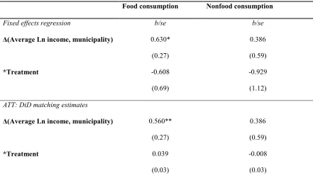
9. Impact of Average Community Income Changes in Household Consumption ... 37
10. Partial Insurance Parameters ... 42
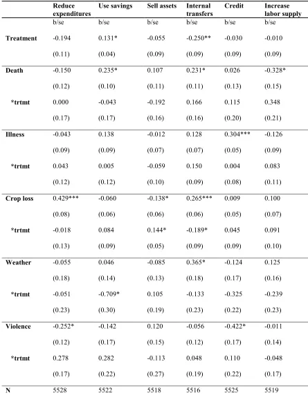
11. Probability of using the following Risk Coping Strategies for Idiosyncratic Income Shocks and the crowding-out effect of FA ... 46
12. Transfers in Money Received by Households ... 47
13. Children’s types of activity, participation percentages ... 63
14. Child labor by group, participation percentages ... 63
15. Children’s time use, number of hours by sex/age groups ... 64
16. Frequency of shocks on households by treatment and control groups ... 66
18. Probability of school enrollment for children 10–17 prior to FA: Fixed effects Probit
Model ... 74
19. Probability of work for children 10–17 prior to FA: Fixed effects Tobit Model ... 75
20. Average treatment effect of FA program for the second round of the survey ... 80
21. Hypothesis of the impact of the CCT program on the labor supply ... 99
22. Summary statistics by treatment group, sample means ... 102
23. Labor force participation prior to the program, percentages ... 104
24. Time allocation of adults, number of hours ... 105
25. Time allocation of children, number of hours... 106
26. Labor force participation of children conditional on attending school ... 107
27. Time allocation of children conditional on attending school ... 108
28. Monthly average income at baseline ... 109
29. Impact of the program on hours of child time uses, Tobit model ... 113
30. Impact of the program on hours of child time uses for children who were attending school prior to the program, Tobit model ... 114
ABSTRACT
THE INDIRECT EFFECTS OF CONDITIONAL CASH TRANSFER PROGRAMS: AN
EMPIRICAL ANALYSIS OF FAMILIAS EN ACCION
By
MONICA OSPINA
May, 2010
Committee Chair: Dr. Ragan Petrie
Major Department: Economics
Conditional cash transfer (CCT) programs have become the most important social
policy in Latin America, and their influence has spread to countries around the world. A
number of studies provide strong evidence of the positive impacts of these programs on
the main targeted outcomes, education and health, and have proved successful in other
outcomes such as nutrition, household income, and child labor. As we expect CCT
programs to remain a permanent aspect of social policy for the foreseeable future,
demand for evidence of the indirect effects of CCT programs has grown beyond the
initial emphasis of these programs. My research pays particular attention to these relevant
but unintended outcomes, which have been discussed less extensively in the literature.
Familias en Accion (FA), a CCT program in Colombia, started operating in 2002
and has benefited approximately 1,500,000 households since its beginning. The results of
the program’s evaluation survey, representative of poor rural households in Colombia, are
also the microeconomic behavior of poor households and social policy issues in the
country. Using a panel dataset from FA, I address three empirical policy questions: (i) to
what extent is consumption of beneficiary households better insured against income
shocks? (ii) has the program displaced child labor as a risk-coping instrument?, and (iii)
are there any incentive effects of the cash transfers and the associated conditionalities on
the labor supply of adults in recipient households?
Each of my research questions is addressed separately; however, the results, taken
together, can be informative in understanding the safety net value of the program and
their potentialities to reduce poverty in the long term. I find that the program serves as an
instrument for consumption smoothing. In particular, FA is effective in protecting food
consumption, but not nonfood consumption, and it reduces consumption fluctuations in
response to idiosyncratic shocks but not to covariate shocks. Results also reveal that FA
works as insurance for the schooling of the poor but is not able to completely displace
child labor. Finally, the results also show that beneficiary mothers are devoting more time
to household chores and that girls and female adult labor are complementary. Male labor
Chapter 1 . CCT PROGRAMS FOR CONSUMPTION INSURANCE: EVIDENCE
FROM COLOMBIA
Introduction
Poor households in developing countries live with high levels of risk and limited
access to formal financial systems for credit and insurance. To secure their levels of
consumption, or smooth consumption, households have traditionally engaged in different
ex-post risk coping strategies; i.e., depletion of assets, increase of labor supply, informal
borrowing, or transfers from relatives. Also, risk-averse households can take ex-ante
actions to mitigate the effects of negative income shocks; i.e., income smoothing.
However, neither of these alternatives allows poor households to achieve an optimal
allocation of risk across time, and most of these strategies are costly in terms of long-term
poverty and vulnerability. In particular, ex-post consumption smoothing strategies might
result in households’ decreased capital accumulation, and the income-smoothing
mechanism might result in reduced investments in productive assets. Thus, the inability
of households to cope with risk is a channel through which they can get into a poverty
trap. For these reasons, the research on risk coping behavior and consumption smoothing
arrangements of poor communities in developing countries is a crucial issue in the
formulation of policies aimed to reduce poverty.
The purpose of this paper is twofold. First, we analyze the degree of consumption
insurance of poor households in Colombia in relation to fluctuations in their incomes due
to idiosyncratic and community shocks.1 Second, we evaluate the effects that a
1
conditional cash transfer program (CCTs), Familias en Acción (FA), has had on
protecting households from the negative effects of shocks. By doing this, we hope to
contribute to the literature of consumption smoothing in developing countries as well as
to provide new evidence of the role of CCTs as risk management instruments. A good
understanding of how and which public interventions provide effective insurance is
crucial for policy design.
Economics literature has broadly studied how individuals smooth consumption in
response to income shocks. Two main hypotheses have dominated the literature. On one
hand, the full risk-sharing hypothesis assumes that consumption is fully insured against
idiosyncratic income shocks but not against community income shocks. On the other
hand, the permanent income hypothesis (PIH) assumes that, under complete credit
markets, self-insurance through borrowing and saving may allow inter-temporal
consumption smoothing against idiosyncratic and covariate shocks. Although both
hypotheses have been rejected repeatedly (e.g., Townsend 1994; Ravallion and
Chaudhuri 1997; Deaton 1992; Skoufias 2003), empirical evidence has shown that
consumption reacts too little to permanent income shocks to be consistent with the
economic theory (Campbell & Deaton, 1989; Attanasio & Pavoni, 2006). Because these
models are extreme characterizations of individual and market behavior, recent literature
has addressed the issue of whether partial consumption insurance is available to agents.
This paper, in addition to following the traditional approach of testing the hypotheses of
complete consumption insurance, estimates partial insurance parameters from the data
In addition to identifying the relationship between consumption smoothing and
income shocks, we give special attention to how public interventions—CCTs, in
particular—can play a significant role in reducing consumption vulnerability of poor
households. According to Morduch (1999), CCTs guarantee that a minimum of insurance
is received in order to compensate for under-provision of safety-net services in poor
areas. There are several ways in which we can expect CCT programs to reduce the risk of
vulnerability: They can (1) reduce income fluctuations because they increase income
irrespective of shocks and thus have the same insurance properties as permanent income;
(2) displace non-desirable coping strategies, such as high-interest loans, child labor, or
depletion of productive assets; (3) create a regulatory and institutional framework to scale
up services through informal safety nets; and (4) counteract the government’s lack of
ability to respond, whether at the central or local level (Cox & Jimenez, 1992).
FA provides subsidies to families on the conditions that all household members
receive periodic health checks and that all children are enrolled in and attend school
regularly. Given the importance of the program at a national level, a rigorous impact
evaluation design has been followed since the very early stages of the program. This has
allowed for the collection of repeated observations of beneficiary households surveyed
before and after the implementation of the program, as well as the collection of similar
data from comparable households that have not been covered by the program. Thus, this
panel dataset provides an excellent opportunity for measuring consumption insurance and
reveals possible roles of public interventions as risk management instruments. This study
has some advantages over other similar studies because of the quasi-experimental design
program’s evaluation survey. First, the balanced panel dataset has detailed information on
consumption, income, and shocks for a representative sample of poor households living
in small villages in Colombia. Most of the datasets used in earlier studies to evaluate
consumption smoothing report either income or consumption, not both. For example, in
order to estimate partial insurance parameters for the United States, Blundell et al. (2008)
have to infer consumption statistically, since consumption and income data are not
available for the same households in a single dataset.
Second, while some studies use changes in income as measures of shocks
(Skoufias, 2003; Townsend, 2004), others use dummy variables for the occurrence of
idiosyncratic shocks in a given period of time (Cochane, 1991; Mace, 1991). Although
income has been criticized as a right hand side variable since it can be endogenous in the
consumption equation (Cochane, 1991), if we are able to control for that endogeneity,
income variance at household and community levels are very informative about the
degree of consumption insurance of poor households. Furthermore, as frequency and
intensity of shock events are difficult to capture in occurrence shocks data, a better
understanding of the vulnerability to shocks is obtained when we are able to complement
these results using income variance and shock events as measures of the risk faced by
these households. The dataset used in this analysis uses both income variance and shock
events to estimate consumption insurance parameters. Finally, as we have data for
treatment and control households before the program was implemented, we are able to
estimate an unbiased effect of the program on consumption smoothing, controlling for
This paper makes three important contributions to the existing literature. First, it
adds to the empirical literature on consumption insurance by providing evidence of the
ability of poor households in Colombia to insure consumption against idiosyncratic and
covariate shocks. Prior evidence of consumption smoothing has been limited to results
from a particular dataset from India2 and a few other samples collected mainly in Asia
and Africa (Baez, 2006). Latin America, a region with a massive proportion of people
living in poverty who are subject to income shocks, is clearly underrepresented in this
literature, in large part due to the lack of suitable information for investigating risk and
insurance of poor households. Second, it contributes to the social program evaluation
literature by going beyond assessing the impact of the program on its main objectives to
analyze the consequences of participation in other dimensions, such as the degree of
informal risk sharing. Third, it is the first paper, to our knowledge, that estimates
consumption insurance parameters under both the full risk-sharing model and a partial
insurance model.
Based on all specifications used in this research, we support estimations from the
partial insurance model as it allows for self-insurance instruments other than savings. We
observe a high, but not complete, level of consumption smoothing among poor
households in small villages in Colombia, with food consumption’s being better insured
than nonfood consumption. In addition, results suggest that FA has been effective as a
risk management instrument protecting food consumption when households are faced by
income shocks and has not displaced risk pooling among households in the same
communities. These findings provide strong indications that households engage in risk
2
management strategies aimed at insulating, at least partially, consumption changes from
income changes. For instance, our results suggest that the introduction of this program
has enforced risk coping instruments such as the use of savings and assets, and has
displaced internal transfers. If FA has in fact crowded-out or enforced existing informal
risk coping strategies and how the final well being of beneficiary households has been
affected are issues not addressed on this paper. Finally, we conclude that FA, despite not
being a consumption insurance program, helps treated families to smooth consumption.
Results are robust to different specifications.
The rest of the paper is organized as follows. The next section provides an
overview of the program and a description of the evaluation sample used for the
empirical analysis. The subsequent section examines risks faced by households in rural
Colombia and describes the data used for the empirical analysis. Following is a section
that presents basic predictions of the full risk-sharing model and the influential findings
on risk coping behavior and consumption smoothing arrangements in developing
economies. The next section contains the empirical model and results for the full
insurance model. The two subsequent sections present the model used in this paper to
estimate partial insurance parameters based on both Blundell et al.’s (2008) and this
study’s estimations, respectively. The following section presents an analysis of risk
coping strategies used by households to buffer adverse income shocks, and the final
Familias en Acción
The program Familias en Acciónis a welfare program run by the Colombian
government to foster the accumulation of human capital in rural Colombia. It is similar to
other CCT programs, such as Progresa, in Mexico (now called Oportunidades); Red de
Proteccion Social, in Nicaragua; and Bolsa Familia, in Brazil, that have been
implemented in middle-income countries during the last decade in an effort to break the
intergenerational transmission of poverty. The FA program is aimed primarily at
improving the education, health, and nutrition of poor families. The nutrition component
consists of a basic monetary supplement that is given to all beneficiary families with
children under seven years of age. The health component consists of vaccinations and
growth and development checks for children, as well as courses on nutrition, hygiene,
and contraception for their mothers. Participation in the health component is a
precondition for receiving the benefits of the nutritional component. All children between
7 and 18 years old are eligible for the educational component. To receive the grant, they
must attend classes during at least 85% of the school days in each school month as well
as during the whole academic year. The size of the grant increases for secondary
education and is equal for girls and boys. The amount of the subsidy on a monthly basis
at the time of the baseline survey was 14,000 Colombian pesos (COP) or (US$6) for each
child attending primary school and COP$28,000 or (US$12) for each child attending
secondary school in 2005. The nutritional supplement3 is paid to families with children
aged between 0 and 6 years. The amount is COP$46,500 or (US$20) per family per
3
month. The average transfer received per household is COP$61,500, which represents
approximately 25% of average household income of beneficiary households. In general,
all the transfers are received by the female head of the household every two months.
Familias en Acción determined household eligibility in two stages: first by
identifying target communities and then by choosing low-income households within
those communities. Selection criteria for target communities were based on the following
conditions. The town must: (i) have fewer than 100,000 inhabitants and not be a
departmental capital, (ii) have sufficient education and health infrastructures, (iii) have a
bank, and (iv) have a municipality administrative office with relatively up-to-date welfare
lists and other official documents deemed important. A subset of 622 of the 1,060
Colombian municipalities qualified for the program. Eligible households were those
registered at SISBEN4 level 1 at the end of December 1999, with children under 17 years
old, living in the target municipalities. SISBEN 1 households account for roughly the
lowest quintile of Colombia’s household income distribution (Attanasio, 2004).
The program started operating in the latter half of 2002.5 It has benefited
approximately 1,500,000 households since its beginning, and the cost has ascended to the
sum of 300 thousands of millions of Colombian pesos annually (US$150 million). The
cost of the program corresponds to the 0.5% of the Colombian GDP and represents
approximately 10% of educational expenditures in the country.
The Evaluation Sample
For evaluation purposes, it was decided to construct a representative stratified
sample of treatment municipalities and to choose control municipalities among those that
4
SISBEN, Sistema Unificado de Beneficiarios, is a six-level poverty indicator used in Colombia to target welfare programs and for the pricing of utilities.
5
were excluded from the program but that belonged within the same strata. The strata were
determined by region and by an index of infrastructure based on health and education.
The control towns were chosen within the same stratum to be as similar as possible to
each of the treatment towns, in terms of population, area, and quality of life index. Most
of the control municipalities were towns with basic school and health infrastructures but
without banks or, in the few cases chosen to match relatively large municipalities, just
over 100,000 inhabitants. As a consequence, control towns are broadly comparable to
treatment towns (Attanasio, 2004). In the end, the evaluation sample was made up of 122
municipalities, 57 of which were treatment and 65 of which were controls.
For each municipality, approximately 100 eligible households were included in
the evaluation sample. The total evaluation sample consists of 11,462 households
interviewed between June and October 2002 (baseline survey), 10,742 households
interviewed between July and November 2003 (first wave), and 9,566 households
interviewed between November 2005 and April 2006 (second wave). The attrition rate
between the three rounds was approximately 16%.6 Most of the observations lost were
households which children´ age exceeded the required age or households that move from
their location and were no possible to find again. Compliance was very high,7 more than
97% of the eligible households participate in the program, so for the analysis we include
in the sample all observations from treatment municipalities.
The final longitudinal data used in this study include information from 6,519
repeated households, after excluding households that received payments before the
6
According to Attanasio (2007) attrition between baseline survey and the second follow up survey is not statistically different between treatment and control households. Therefore we assume that lost of observations is random.
7
baseline survey and households located in control municipalities that received payments
during the second survey. 8 At the household level, the sample consists of families that
are potential beneficiaries of the program—that is, households with children from the
poorest sector of society. Data are collected at both the household and the individual
level. The available data provide a rich set of variables that allows us to measure
consumption of durables and non-durables, family composition, household
socio-demographic structure, labor supply, nutritional status of children, education, household
assets, income, and different shocks to income, for both rural and urban households.
Empirical Evidence on Risk and Consumption
Shocks
The variables used to identify the various shocks experienced by households are
obtained from direct questions in the evaluation survey. In each of the three survey
rounds, the household was asked whether during the last year it had experienced any of
the following shocks: crop loss or job loss, death of a household member, illness of any
household member, violent attack or displacement, or weather shock.9 We include an
additional shock, unemployment of the household head, which takes a value of one if the
household head was looking for a job for more than three months during the year
previous to the survey. In that way, we expect to capture a severe income shock.
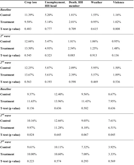
For the sample of households in treatment and control municipalities, the
prevalence of different types of shocks at the household level during each of the
cross-section surveys are reported in Table 1. As we observe, there is no statistical difference
8
A total of 13 municipalities of the control sample were converted to treatment municipalities in 2005, before the second wave of the evaluation survey.
9
between treatment and control households for all of the shocks, except for illness during
the first round. In order to control for potential endogeneity of this shock, we distinguish
between illnesses of children, which can be very endogenous, and illnesses of the
household head and other adults, which should be less endogenous. Participation in the
program could decrease the vulnerability to disease shocks of children, as the program
imposes regular visits to health centers as a condition for receiving part of the transfers
(Attanasio, 2004). We find that illness of the household head is not statistically different
between treatment and control municipalities, suggesting that it is an exogenous shock,
while illness of children and spouse are correlated with program participation and so
might be endogenous. For the purposes of this research we use exclusively illness of
household head as a measure of shock.
Data show that the exposure of households to crop loss and unemployment of
household head is very high: over 10% of households had at least one crop loss and over
5% had at least one member unemployed for more than 3 months during the year
previous to the interview. Around 11% of the households reported having the household
head ill for more than two weeks at least once over the year prior to the survey. Death of
any household member, being a victim of violence, and weather shocks are less frequent
but can be very harmful to poor families because they result not only in loss of income
Table 1. Frequency of Idiosyncratic Shocks
Crop loss Unemployment,
HH head
Death, HH member
Weather Violence
Baseline
Control 11.39% 5.20% 1.81% 1.55% 1.16%
Treatment 9.58% 5.14% 2.01% 0.95% 1.02%
T-test (p value) 0.483 0.777 0.709 0.615 0.808
1st wave
Control 12.66% 5.47% 1.81% 1.06% 0.95%
Treatment 13.50% 4.93% 2.54% 1.25% 1.48%
T-test (p value) 0.545 0.323 0.085 0.913 0.136
2nd wave
Control 12.25% 5.87% 2.09% 5.95% 1.50%
Treatment 13.67% 5.61% 2.39% 5.57% 1.89%
T-test (p value) 0.563 0.193 0.598 0.469 0.536
Baseline
Control 9.37% 12.40% 9.56% 8.67%
Treatment 11.65% 13.96% 11.43% 7.95%
T-test (p value) 0.136 0.636 0.582 0.636
1nd wave
Control 10.16% 12.66% 9.05% 7.61%
Treatment 9.97% 11.28% 8.18% 6.51%
T-test (p value) 0.024 0.645 0.067 0.045
2nd wave
Control 9.61% 10.11% 7.32% 3.92%
Treatment 10.00% 10.60% 7.08% 3.33%
T-test (p value) 0.223 0.574 0.293 0.569
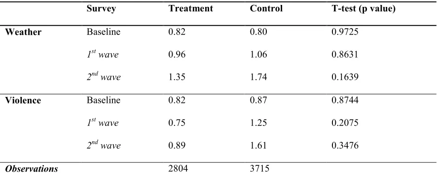
In order to capture the covariate nature of weather shocks, we use the proportion
of households within a municipality reporting to have suffered this shock (de Janvry et
al., 2006). Community violence is obtained from other sources and measures the number
of terrorist attacks that municipalities had during the year before the interview.10 Mean
statistics and differences among treatment and control municipalities are presented in
Table 2. As we can observe, there are not pre-treatment and post-treatment statistical
differences in the occurrence of these covariate shocks between treatment and control
[image:25.612.103.546.319.505.2]municipalities.
Table 2. Frequency of Covariate Shocks
Survey Treatment Control T-test (p value)
Weather Baseline 0.82 0.80 0.9725
1st wave 0.96 1.06 0.8631
2nd wave 1.35 1.74 0.1639
Violence Baseline 0.82 0.87 0.8744
1st wave 0.75 1.25 0.2075
2nd wave 0.89 1.61 0.3476
Observations 2804 3715
otes: Numbers indicates the average proportion of households on each municipality that have suffered
weather and violence shocks. T-test of difference in means among communities in the sample.
Consumption
The evaluation survey of FA contains detailed information on food and nonfood
expenditures in all three rounds: baseline, first wave, and second wave. In food
expenditures, there is information on the amount of money spent by households in buying
10
fruits and vegetables, cereals and grains, meats and animal products, and other food
products, like soft drinks, alcoholic beverages, coffee, tea, etc. In the nonfood
expenditures category, there is information on the money spent on clothing, health
products and services, house maintenance products, school and educational goods,
transportation, utilities, and other nonfood expenditures, like cigarettes, social events, and
toys. Expenditures on durables, such as furniture, and luxury items are excluded from our
expenditure measures as they not represent a regular expenditure of the household.
Depending on the commodity, good, or service, the survey asked the head of
household about the expenditures made during the week, month, semester, or year prior
to the date of the survey. In order to construct the measures of household consumption
used in this paper, we converted all expenditures into a household’s monthly
expenditures and then added them up across the corresponding categories: total
consumption, food consumption, and nonfood consumption. We also deflated the
measures using the National Consumer Price Index of Colombia and turned them into
adult-equivalent11 pesos at constant 2002 prices. In-kind food consumption12is included in
our measures using town-level prices observed for households buying similar commodities.
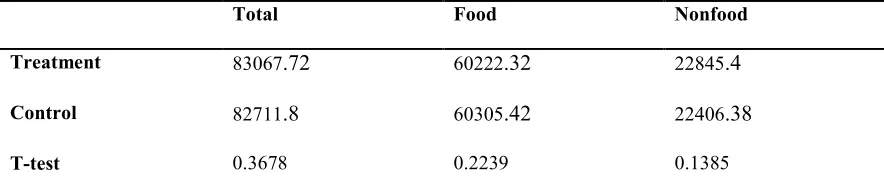
Table 3 shows that households spend around COP$8,000 per adult equivalent per
month on total consumption, and that 70% of these expenditures are on food. There are
no pretreatment differences in consumption between treatment and control households.
Attanasio et al. (2005) have shown the effectiveness of the FA program to increase food
consumption in both rural and urban areas. They estimate a 15% increase in average
consumption levels one year after the baseline survey. They also find that shares in food
11
Household members older than 12 years old are counted as 1 person; household members younger than 12 years are counted as 0.5 person.
12
and nonfood consumption are not affected by the program but that it has created
redistributive effects in favor of children through expenditure on children’s clothing and
on education. They also found that the program has not significantly affected
[image:27.612.103.545.210.306.2]consumption of adult goods, such as alcohol and tobacco or adults’ clothing.
Table 3. Consumption at Baseline
Total Food &onfood
Treatment 83067.72 60222.32 22845.4
Control 82711.8 60305.42 22406.38
T-test 0.3678 0.2239 0.1385
otes: Consumption measures are per adult equivalent deflated to 2002 price level in Colombian pesos.
T-test of difference in means computed clustering at the municipality level.
Control Variables
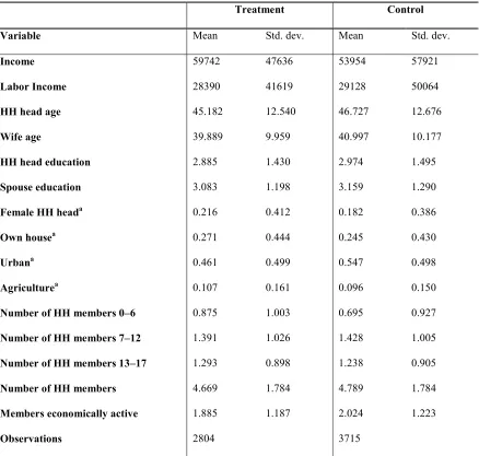
Table 4 provides the means and standard deviations of the main variables used in
the analysis for the sample of households in the treatment and control municipalities for
all three surveys. All of the variables used in all of the regressions are at the household
level. Monthly household income is constructed by adding reported labor income,
self-employment, pensions, interest, rents, and government transfers, including FA potential
transfer.13 Income transfers and remittances received from neighbors, friends, and
relatives are excluded from total income, as these sources of income are likely to reflect
ex-post adjustments to shocks. Income is expressed in adult equivalent measures and
deflated to 2002 prices. Agriculture indicates the household head was occupied in
agricultural activities. Members economically active indicates the number of persons in
13
the household older than 12 who were working or looking for job at the moment of the
survey. Education variables indicates the last level of education by the head and partner
of the household.14Urban is a dummy variable that takes a value of one for households
located in urban areas and zero, otherwise. Household composition variables represents
the proportion of household members by age.
14
Table 4. Summary Statistics of Main Variables for all Survey Rounds
Treatment Control
Variable Mean Std. dev. Mean Std. dev.
Income 59742 47636 53954 57921
Labor Income 28390 41619 29128 50064
HH head age 45.182 12.540 46.727 12.676
Wife age 39.889 9.959 40.997 10.177
HH head education 2.885 1.430 2.974 1.495
Spouse education 3.083 1.198 3.159 1.290
Female HH heada 0.216 0.412 0.182 0.386
Own housea 0.271 0.444 0.245 0.430
Urbana 0.461 0.499 0.547 0.498
Agriculturea 0.107 0.161 0.096 0.150
&umber of HH members 0–6 0.875 1.003 0.695 0.927
&umber of HH members 7–12 1.391 1.026 1.428 1.005
&umber of HH members 13–17 1.293 0.898 1.238 0.905
&umber of HH members 4.669 1.784 4.789 1.784
Members economically active 1.885 1.187 2.024 1.223
Observations 2804 3715
otes: Averages based on three rounds. Income measures are per adult equivalent deflated to 2002 price
level in Colombian pesos.a Mean values of dummy variables represent percentage of households that meet
each of the conditions of the variables.
Full Risk Sharing and the Permanent Income Hypothesis
The most relevant risk coping strategies theorized in the literature are the full
risk-sharing hypothesis and the permanent income hypothesis (PIH). The full risk-risk-sharing
consumption would be independent of any idiosyncratic shock affecting the income
available to the household (Bardhan & Udry, 1999). That is, the only risk that any
household faces is the risk faced by the municipality as a whole. The alternative
mechanism to coping with income shocks is the permanent income hypothesis, which
states that a household with no opportunity for cross-sectional risk pooling, but with
unlimited access to a credit market and separable preferences of consumption and labor,
makes savings or lending decisions so that the effects of shocks are spread out between
current and future consumption (Bardham & Udry, 1999). According to the hypothesis,
individuals tend to smooth consumption when facing transitory income fluctuations. In
practice, these hypotheses are not very relevant to most of the rural households in
developing countries, given the inexistence of complete credit markets.
Although both hypotheses have been repeatedly rejected in studies using
micro-data, empirical evidence has shown that consumption reacts too little to income shocks to
be consistent with the theory. Townsend (1994) and Ravallion and Chaudhuri (1997) test
the hypothesis in the ICRISAT Indian villages and reject it, although they find a
substantial amount of risk sharing. Deaton (1992) and Grimard (1997) test the hypothesis
of perfect risk sharing within villages and ethnic groups in Côte d’Ivoire and find little
evidence of any risk pooling at the municipality level and somewhat stronger evidence
within ethnic groups. Udry (1994) also rejects the hypothesis for northern Nigerian
villages. Skoufias (2003) examined the extent to which Russian households were able to
protect their consumption from fluctuations in their income using longitudinal data from
idiosyncratic shocks to income; with food consumption’s being better protected than
nonfood consumption expenditures.
Evidence from developed countries has also rejected the hypothesis of full risk
insurance (Mace, 1991; Cochrane, 1991). Cochrane (1991), using data on household food
consumption from the Panel Study of Income Dynamics (PSID) for the period 1980–
1983, regressed changes in consumption onto different measures of idiosyncratic shocks.
His results rejected the full insurance hypothesis for some but not all of the different
shocks. Similarly, Mace (1991) tested consumption insurance with panel data from the
U.S. Consumer Expenditure Survey (CEX). She could not reject the full insurance
hypothesis when evaluating changes in consumption against changes in income, but she
did reject full insurance when using growth rates. Finally, using household panel data
from Bangladesh, Ethiopia, Mali, Mexico, and Russia, Skoufias and Quisumbing (2003)
examined the extent to which households are able through formal and/or informal
arrangements to insure their consumption from specific economic shocks and fluctuations
in their real income. The study showed that adjustments in nonfood consumption
appeared to act as a mechanism for partially insuring ex-post the consumption of food
from the effects of income changes.
These findings raise the question of how households achieve some level of
consumption smoothing given their limited access to financial markets. It seems that poor
households engage in self-insurance strategies and mechanisms to secure their level of
consumption once they face negative shocks. The most common self-insurance
mechanisms for uninsured households are taking loans from the informal financial sector
household labor supply (Kochar, 1998), or sending children to work in order to
supplement income (Jacoby & Skoufias, 1997). Townsend (1994) showed that even
extremely poor villages in rural India may have self-insurance strategies that allow them
to come close to an optimal allocation of risk bearing. While these actions enable
households to spread the effects of income shocks over time, they might have adverse
consequences in the long run in terms of poverty and future vulnerability of households.15
According to Baez (2006), the work to date on the extent of consumption
smoothing in rural areas allows us to draw three important conclusions. First, most if not
all of the empirical work has mainly rejected the full risk-sharing model. Second, and
regardless of that rejection, a large amount of consumption smoothing is taking place.
Rural households are not purely consuming what they earn, although the poorest have
less scope to do so. And third, considering some market failures that obstruct formal
insurance in rural villages, informal mechanisms seem to play a significant role in
protecting their consumption.
As these conclusions have been widely accepted, recent literature has gone
beyond the complete market model and has proposed and encouraged “the construction
and testing of market models with partial insurance” (cited in Blundell et al., 2008;
Deaton & Paxson, 1992). Also, literature has centered on alternative informal instruments
to bear risk, estimating the extent of consumption insurance over and above
self-insurance, including the role of public interventions. In this paper we address both issues.
First, we investigate how well-known public interventions in developing countries—
15
CCTs—can play a significant role in reducing consumption vulnerability of poor
households. Second, we estimate the degree of consumption insurance under the full
risk-sharing model and under a partial insurance model recently proposed by Blundell et al.
(2008).
Public interventions can play a significant role in strengthening or displacing the
informal insurance mechanisms already in place. The following examples illustrate some
of the effects of public intervention on consumption insurance. In South Africa, Jensen
(2002) compares the difference in the level of remittances received by pensioned and
non-pensioned workers, after the increase in pension levels, relative to the difference
before the increase. Findings based on the crowding-out effect differ across both groups.
In Mexico, public cash transfer programs have not displaced informal mechanisms within
the scheme of risk-sharing mechanisms (Skoufias, 2003); the evidence, however, is not
clear for Northern Thai villages, where the effects of public intervention vary across
distinct private transfers and informal mechanisms (Townsend, 1995). Finally, in the case
of Mexico, García-Verdú (2002) analyzes a model of informal insurance and also finds
that there is no crowding-out effect between cash transfers and informal safety nets.
To date, no structural model has been estimated to address the issue of partial
insurance directly. Blundell et al. (2008) address the issue of whether partial consumption
insurance is available to agents and estimate the degree of insurance over and above
self-insurance through savings. They do so by contrasting shifts in the distribution of income
growth with shifts in the distribution of consumption growth and then analyze how these
two measures correlate over time. We follow this methodology to estimate the parameters
proposed by Blundell et al. (2008), which is used in this paper for the estimation of
partial insurance parameters.
Empirical Evidence of Consumption Insurance under the Full Risk-sharing Model
In this section we consider the model of Pareto efficient risk pooling within a
community to estimate the extent of risk sharing in poor households in Colombia and to
test the effect of FA as an instrument for consumption smoothing. One way of testing the
hypothesis of complete risk sharing within a community is to examine whether the
growth rate of household consumption is independent of the growth rate in household
income after controlling for aggregate shocks. We employ the following specification
commonly encountered in the literature (e.g., Cochrane, 1991; Mace, 1991; Townsend,
1994; Ravallion & Chaudhuri, 1997). 16
= + + ∗ + + + + + + + (1)
where C refers to adult equivalent consumption per capita of household i in
municipality v at time t; Srepresents idiosyncratic shocks; FA is a dummy for
households that participate in the program; Xis a set of socioeconomic and
demographic characteristics of the household that takes into account the composition of
the household by age, sex, and education level of household head; and
δ,γ,µ,τandεrepresent household, municipality, time, municipality-time
fixed-effects, and the idiosyncratic error term, respectively.
Theory predicts that, under complete risk sharing, = 0, and provides an
estimate of the extent to which idiosyncratic income shocks play a significant role in
16
explaining the household-specific consumption changes. For the purposes of the
empirical analysis, the insurance group is defined to be the full set of households within a
municipality.17 Since our sample is representative of poor households in small towns in
Colombia, and credit and insurance markets don’t function at all in these towns,18 the
identification of the insurance group is adequate. In addition, we should expect that
insurance arrangements are easier to organize and enforce in small and poor
communities.
To test the effect of FA on consumption smoothing of beneficiary households,
equation (1) include FAht, which is abinary variable equal to 1 for households in
treatment municipalities for the first and second follow-up surveys, and 0 for households
in control municipalities in all three surveys and for treatment municipalities at baseline.
In this equation, the coefficient is the difference in the vulnerability to risk between
beneficiary and control households in the program that have been hit by the same shock.
A negative estimate of α implies that FA has decreased vulnerability to risk in the
treatment communities. An insignificant estimate of αsuggests that there are no
significant differences in the level of consumption insurance between control and
treatment households. The coefficient reflects the effect of the program on
consumption for households that have been hit by each of the income shocks considered.
Since the program was not randomly assigned among participants and control
households, we can expect program participation being endogenous on the consumption
equation. However, we found balance between the covariates for each sub-sample19 so
we assume that program participation is not correlated with the unobservable
17
On average, there are 50 households in each municipality.
18 Less than 5% of the households have credit or a savings account.
characteristics on the consumption equation. In addition, using fixed effects regressions
we are able to control for unobservable time invariant characteristics. Alternatively, we
used matching methods to find control households comparable to treatment households.
Results from matching are very similar to results without matching for crop loss and
illness of the household head, and matching was not possible for death and
unemployment shock events. Therefore, we show results from fixed effect regressions.
We consider different definitions of consumption and different types of
idiosyncratic shocks to estimate fixed effects regressions. As dependent variables we use
food consumption, nonfood consumption, and total consumption. The idiosyncratic
shocks considered are: (i) death of a household member, (ii) illness of the household
head, (iii) crop loss or job loss, and (iv) unemployment of household head. The
household surveys asked each household whether it has suffered any of these shocks
during the year prior to the date of the interview. Hence, each household was allowed to
declare whether it was affected by a shock or not.
Fixed effects estimates of equation (1) presented in Table 5 include estimations
for one type of shock at a time, and households hit by one shock, two shocks, and three or
more shocks.20 As discussed above, these estimates are obtained under the assumption
that the insurance group consists of all households in a municipality and include
municipality-year fixed effects. All regressions control for household composition by
age, sex, and the following household characteristics: age and dummies for level of
education of the household head, female household head, number of household members
20
active in the labor market, dummy if the house is owned as a measure of assets, dummy
for households working in agriculture as a proxy of vulnerability to shocks, and
municipality characteristics such as population, number of schools and health centers,
dummy for households located in urban regions as well as in different economics regions
[image:37.612.105.545.239.644.2]in the country.
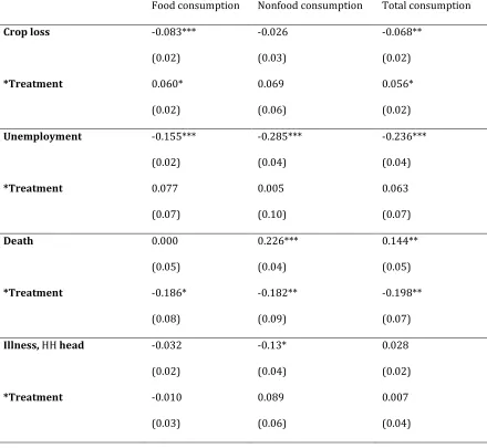
Table 5. Impact of Idiosyncratic Shocks on Consumption: fixed effects estimation
Food consumption Nonfood consumption Total consumption
Crop loss -0.083*** -0.026 -0.068**
(0.02) (0.03) (0.02)
*Treatment 0.060* 0.069 0.056*
(0.02) (0.06) (0.02)
Unemployment -0.155*** -0.285*** -0.236***
(0.02) (0.04) (0.04)
*Treatment 0.077 0.005 0.063
(0.07) (0.10) (0.07)
Death 0.000 0.226*** 0.144**
(0.05) (0.04) (0.05)
*Treatment -0.186* -0.182** -0.198**
(0.08) (0.09) (0.07)
Illness, HH head -0.032 -0.13* 0.028
(0.02) (0.04) (0.02)
*Treatment -0.010 0.089 0.007
Food consumption Nonfood consumption Total consumption
One shock -0.046** -0.112*** -0.065***
(0.02) (0.03) (0.02)
*Treatment 0.031* 0.061* 0.038*
(0.01) (0.04) (0.02)
Two shocks -0.046** -0.135*** -0.095***
(0.02) (0.03) (0.02)
*Treatment 0.021* 0.028 0.058
(0.01) (0.04) (0.09)
Three shocks -0.040** -0.149*** -0.105***
(0.02) (0.03) (0.02)
*Treatment 0.010* 0.061 0.049
(0.01) (0.04) (0. 13)
otes: The measure of consumption is its adult equivalent value in units of 2002 pesos. Estimations are
marginal effects of the control variables of interest, ie. Shock events. Robust standard errors, clustered at
the municipality level, are in parentheses. Additional repressors included but not reported: household age
and education, household composition by age and sex, number of household members active in the labor
market, if the house is owned, if household members work in agriculture, and municipality characteristics
such as population, number of schools and health centers, if urban. Total number of observations is
6519.Municipality-year effects included. Each individual coefficient is statistically significant at the *10%,
**5%, or ***1% level.
Considering shocks one at a time, it is evident that the null hypothesis of perfect
risk sharing is rejected for crop loss, unemployment and illness of the household head.
Crop loss will reduce per capita food consumption by 8% and total consumption by 6%,
28%.21 Illness of the household head reduces nonfood consumption by 13% and doesn´t
have a significant effect on food consumption. Death of a household member increase
nonfood and total consumption with respect to households that have no shocks, so there
is no evidence of consumption smoothing for this shock. The increase in nonfood
consumption is explained by the fact that these shocks usually increase funeral
expenditures.22
The role of FA as an instrument for consumption insurance is also evaluated.
Being a beneficiary of the FA program would protect the household’s food consumption
when it experiences a crop loss but not unemployment of the household head. That is,
while control households reduce food consumption by 8% when they have a crop loss,
treatment households reduce food consumption by 2%. It is interesting to see that
treatment households are no better insured against unemployment than control
households as the estimated coefficient is not statistically different from zero. Negative
estimations of death shocks for treatment households indicate that, while control
households increase non food consumption after these shocks, treatment households are
better able to buffer them. One explanation is that treatment households might have
available less costly ex-ante self-insurance strategies than control households. For
example, it is possible that the FA cash transfer works also as an income-smoothing
mechanism for treatment households.
21
The high coefficients of job loss could be a consequence of the potential endogeneity of this variable in the consumption equation. It could be expected that unemployment is correlated with unobservable characteristics of the household to explain consumption.
22
Finally, we measure the effect of having one shock and having more than one
shock at a time.23 Having a negative shock reduces food consumption by 4% and non
food consumption by 11%, and the program partially protects food and non food
consumption. Having two or more shocks reduces food by 4% and non food consumption
by 14% and the program FA partially protects food consumption but non food
consumption. There are not big differences in consumption changes between having two
or more shocks.
Covariate Shocks
In order to capture the covariate nature of weather and violence shocks, we use
the proportion of households within a municipality reporting to have suffered each shock
as environmental and violence shock variables. Also, we use an alternative measure for
violence: the number of terrorist attacks that municipalities have had during the year
before the interview.
To examine the degree of consumption smoothing of individual households with
respect to covariate risk, we remove the municipality-year fixed effects from the
estimation to calculate the following equation:
= + ' + '∗ + '+ + + + + (2)
The model of full risk sharing predicts that local risk-sharing arrangements permit
households to efficiently pool the idiosyncratic variation within communities, but they
can do little to help households deal with covariate risk. .. Therefore, we should expect
' = 1, under a Pareto efficient model, or an estimate of 0 < ' < 1 if households are
23
able to smooth at least some part of community shocks by formal or informal insurance
mechanisms.
As before, we consider the following dependent variables: food consumption,
nonfood consumption, and total consumption. The covariate shocks considered are: (i)
violence and (ii) weather shocks. For estimation, we use fixed effects regression with
robust standard errors clustering at a municipality level. All regressions control for the
same exogenous variables included in equation (1).
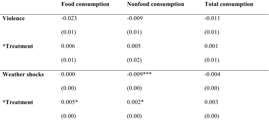
Results are presented in Table 6. As we observe, violence does not affect
consumption. This is reasonable if we assume that most of the terrorist attacks are
targeted at institutions such as banks, police stations, government offices, or to the army
and not to civilians. Weather shocks seem to have a very small effect on consumption,
decreasing nonfood consumption by 0.91% in control communities and by only 0.71% in
treatment communities. Results are opposite to economic predictions, under which we
should expect a positive and significant effect from covariate shocks on consumption,
with estimations close to one. However, these results can be explained by the fact that
they are not permanent but transitory shocks. In fact, Colombia had no severe long-term
Table 6. Impact of Covariate Shocks on Consumption: fixed effects regression
Food consumption &onfood consumption Total consumption
Violence -0.023 -0.009 -0.011
(0.01) (0.01) (0.01)
*Treatment 0.006 0.005 0.001
(0.01) (0.02) (0.01)
Weather shocks 0.000 -0.009*** -0.004
(0.00) (0.00) (0.00)
*Treatment 0.005* 0.002* 0.003
(0.00) (0.00) (0.00)
otes: The measure of consumption is its adult equivalent value in units of 2002 pesos. Estimations are
marginal effects of the control variables of interest, ie. community shock events. Robust standard errors,
clustered at the municipality level, are in parentheses. Additional repressors included but not reported:
household age and education, household composition by age and sex, number of household members active
in the labor market, if the house is owned, if household members work in agriculture, and municipality
characteristics such as population, number of schools and health centers, if urban. Municipality-year effects
included. Total number of observations is 6519.Each individual coefficient is statistically significant at the
*10%, **5%, or ***1% level.
Consumption Smoothing Against Idiosyncratic Income Change
Most of the empirical studies (Skoufias, 2003; Townsend, 1994; Ravallion &
Chaudhuri, 1997) have tested the hypothesis of full risk sharing using changes on
household income as a measure of shocks. Using income growth instead of negative
shocks dummy variables has the advantage that income has the same time frame as
consumption. In the section above, the reference period of consumption (the month
We estimate equation (3) using a fixed effects regression and DID matching
regression in order to control for potential endogeneity of program participation on the
consumption equation.24 In this specification we use consumption growth per adult
equivalent in constant values as a dependent variable and income growth per adult
equivalent in constant values as independent variables. Since declared income might be
endogenous in our specifications, we use lagged income as instrumental variables of
income.25 Municipality-time fixed effects are replaced by a set of binary variables D
identifying each community separately by survey round (round and community
interaction terms). Including the community/round interaction dummies have the purpose
of controlling for aggregate shocks insured at the community level.
∆= + ∆*+ ∗ ∆*+ + + ∑ ,+ (3)
Results from this specification will reveal the average degree of consumption
insurance in the community to any change in the household’s income. As before, under
full risk sharing we expect α = 0, but if α is positive and significant, it provides an
estimate of the partial correlation between income and consumption growth in control
municipalities. If FA helps beneficiary households to cope with income shocks, we
should expect a significantly negative estimate of α, and the sum α + α will provide
an estimate of the partial correlation between income and consumption growth in the
treatment municipalities. The measure of consumption insurance adopted under this
specification can be interpreted as a partial insurance parameter, where lower estimated
24
Using DID matching gave us an advantage over the small number of studies that have tried to identify the impact of cash transfer programs on consumption insurance. As Skoufias (2003) remarks, “the absence of any reliable consumption data in treatment and control villages before the implementation of Progresa prevent one from applying the difference-in-differences estimator for the evaluation of the impact of PROGRESA on consumption insurance” (pp.638).
25
values of α suggest a high degree of consumption insurance and thus a lower
vulnerability of consumption to income shocks (Amin et al., 2003).
In order to correct any pretreatment differences remaining from the
quasi-experimental design used to select the sample of treatment and control municipalities, we
also use a difference in difference matching estimator26 (also called conditional
matching) to estimate the effects of the program in consumption for households with
income shocks. . Matching involves pairing treatment and comparison units that are
similar in terms of their observable characteristics, and a DID estimator compares the
conditional before/after outcomes of participants with those of nonparticipants, allowing
for unobservable but temporally invariant differences in outcomes between participants
and nonparticipants. Thus, the DID matching estimator extends the conventional DID
estimator by defining outcomes conditional on the propensity score and using
nonparametric matching methods to construct the differences. DID matching is superior
to DID as it does not impose linear functional form restrictions in estimating the
conditional expectation of the outcome variable (Smith & Todd, 2005).
For matching, we use non-parametric kernel propensity score matching with
replacement to find the best counterfactual sample, and then estimate the difference in
difference equation. We use the Imben´s variance matrix to estimate the statistically
significance of the estimated ATT. Finally, we restrict the analysis to individuals in the
common support27 in order to minimize any bias due to extrapolation within the
parametric specification and reweight the observations according to the weighting
26 DID matching was first suggested by Heckman et al. (1998a). It extends the conventional DID
estimator by defining outcomes conditional on the propensity score and using semiparametric methods to construct the differences.
27
function of the matching estimator. We also estimate the bias-corrected matching
estimator proposed by Imbens (2004) which adjusts the difference within the matches for
the differences in their covariate values. Finally, since our treatment households are those
eligible on the program, our estimations represent intent to treat effect of the program on
the treated (ITT). However, we expect this is very close to the average treatment effect of
the program (ATT) as non-compliance was mainly due to lack of required documents of
the households.
Estimations of equation (3) using fixed effects regression are reported in Table 7
and in Table 8 using DiD Matching regression. Results show that, when we measure
shocks as changes in income, matching is required in order to control for potential
differences between treatment and control households on consumption. The estimates
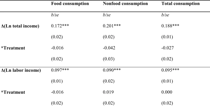
presented in Table 7 column (1) show that a 10% drop in real income is accompanied by
a 1.8% drop in household total consumption, a slightly lower (1.7%) decrease in food
consumption, and a higher (2%) drop in nonfood consumption. However, the
insignificant coefficients of the interaction of income changes with the dummy variable
identifying beneficiary households of FA suggest that there are no significant differences
in the level of consumption insurance between control and treatment households. The
effect of the program is better identified using matching methods. Results in Table 8
show that, controlling for pretreatment differences, FA partially insures food
consumption but not nonfood consumption. Unbiased estimates of the impact of the
program on consumption insurance improve our previous estimates and are robust with
The same regression was estimated using percentage change in labor income as an
explanatory variable. We should expect a higher degree of consumption insurance with
respect to changes in labor income than with respect to changes in total income since
labor income is already insured.28 In fact, we observe in Table 7 and Table 8 that
consumption insurance is higher for labor income than for total income. The estimates for
food consumption indicate that a 10% decrease in labor income will reduce total
consumption by 0.9%, with no differences between food and nonfood consumption.
Estimations using matching methods are very similar to estimations using fixed effect
[image:46.612.106.545.403.633.2]regression.
Table 7. Fixed Effects Regression: Impact of Household Income Changes in Household
Consumption
Food consumption &onfood consumption Total consumption
b/se b/se b/se
∆(Ln total income) 0.172*** 0.201*** 0.188***
(0.02) (0.02) (0.01)
*Treatment -0.016 -0.042 -0.027
(0.02) (0.03) (0.02)
∆(Ln labor income) 0.097*** 0.090*** 0.095***
(0.01) (0.02) (0.01)
*Treatment -0.016 0.019 0.000
(0.02) (0.02) (0.02)
otes: The measure of consumption is its adult equivalent value in units of 2002 pesos. Estimations are the
marginal effects of being a FA beneficiary and having an income shock. Robust standard errors, clustered
28
at the municipality level, are in parentheses. Additional repressors included but not reported: household age
and education, household composition by age and sex, number of household members active in the labor
market, if the house is owned, if household members work in agriculture, and municipality characteristics
such as population, number of schools and health centers, if urban. Municipality-year effects included.
Total number of observations is 6519.Each individual coefficient is statistically significant at the *10%,
[image:47.612.107.544.292.527.2]**5%, or ***1% level
Table 8. DID Matching Estimations: Impact of Household Income Changes in Household
Consumption Controlling for Pretreatment Effects
Food consumption &onfood consumption Total consumption
b/se b/se b/se
∆(Ln total income) 0.237*** 0.257*** 0.234***
(0.02) (0.02) (0.01)
*Treatment -0.139*** -0.008 -0.154
(0.03) (0.03) (0.05)
∆(Average Ln labor income)
0.094*** 0.093*** 0.095***
(0.01) (0.02) (0.01)
*Treatment -0.031 -0.021 0.000
(0.02) (0.02) (0.02)
otes: The measure of consumption is its adult equivalent value in units of 2002 pesos. Estimations are the
ATT on consumption of being a FA beneficiary controlling for household income shocks. Robust standard
errors, clustered at the municipality level, are in parentheses. Additional repressors included but not
reported: household age and education, household composition by age and sex, number of household
members active in the labor market, if the house is owned, if household members work in agriculture, and
municipality characteristics such as population, number of schools and health centers, if urban.
Municipality-year effects included. Total number of observations is 6519.Each individual coefficient is