New insights into the differences between the dual node approach and the common node approach for coupling surface–subsurface flow

https://doi.org/10.5194/hess-21-5709-2017 © Author(s) 2017. This work is distributed under the Creative Commons Attribution 3.0 License.

New insights into the differences between the dual node

approach and the common node approach for coupling

surface–subsurface flow

Rob de Rooij

Water Institute, University of Florida, 570 Weil Hall, P.O. Box 116601, Gainesville, FL-32611-6601, USA

Correspondence to:Rob de Rooij ([email protected])

Received: 21 March 2017 – Discussion started: 30 March 2017

Revised: 10 October 2017 – Accepted: 11 October 2017 – Published: 17 November 2017

Abstract. The common node approach and the dual node approach are two widely applied approaches to coupling surface–subsurface flow. In this study both approaches are analyzed for cell-centered as well as vertex-centered finite difference schemes. It is shown that the dual node approach should be conceptualized and implemented as a one-sided first-order finite difference to approximate the vertical sub-surface hydraulic gradient at the land sub-surface. This results in a consistent dual node approach in which the coupling length is related to grid topology. In this coupling approach the coupling length is not to be interpreted as a nonphysical model parameter. Although this particular coupling approach is technically not new, the differences between this consistent dual node approach and the common node approach have not been studied in detail. In fact, this coupling scheme is often believed to be similar to the common node approach. In this study it is illustrated that in comparison to the common node approach, the head continuity at the surface–subsurface inter-face is formulated more correctly in the consistent dual node approach. Numerical experiments indicate that the consistent dual node approach is less sensitive to the vertical discretiza-tion when simulating excess infiltradiscretiza-tion. It is also found that the consistent dual node approach can be advantageous in terms of numerical efficiency.

1 Introduction

There is a variety of hydrogeological problems, such as the hydrologic response of hillslopes and river catchments, which requires an integrated analysis of surface and

sub-surface flows. This has led to the development of phys-ically based, distributed parameter models for simulating coupled surface–subsurface flows. Well-known examples of such models include MODHMS (Panday and Huyakorn, 2004), InHM (Ebel et al., 2009), HydroGeoSphere (Therrien et al., 2010), CATHY (Camporese et al., 2010), WASH123D (Yeh et al., 2011), ParFlow (Kollet and Maxwell, 2006) and OpenGeoSys (Kolditz and Shao, 2010). Typically, subface flow is governed by the Richards’ equation whereas sur-face flow is either governed by the kinematic wave or the diffusive wave equation.

a very small coupling length (Ebel et al., 2009; Liggett et al., 2012, 2013). Since it is known that the dual node ap-proach mimics the common node in the limit as the cou-pling length goes to zero (Ebel et al., 2009), it thus seems that the dual node approach is most accurate if it mimics the common node approach. Nonetheless, it has been argued that the dual node approach remains an attractive alternative cou-pling approach since it offers more flexibility than the com-mon node approach. Namely, while it can mimic the comcom-mon node approach, the dual node approach offers the possibility to simulate a less tight coupling of surface–subsurface flow which results in increased computational efficiency (Ebel et al., 2009).

In this study a detailed analysis of both coupling ap-proaches is provided for cell-centered as well as vertex-centered finite difference schemes. This analysis starts with the crucial observation that the topmost subsurface nodal val-ues as computed by the finite difference schemes represent the mean values within the topmost discrete control volumes. Numerical experiments to compare the coupling approaches are carried out with the model code DisCo (de Rooij et al., 2013b). It is shown that the dual node approach should be interpreted and implemented as a one-sided finite difference approximation of the vertical hydraulic gradient at the land surface. This yields a consistent dual node scheme in which the coupling length is defined by the half the thickness of the topmost subsurface cells. The scheme of An and Yu (2014) as well as the scheme of Kumar et al. (2009) are essentially very similar to this consistent dual node scheme. In the work of Panday and Huyakorn (2004), one of the suggestions to define the coupling length is to use half the thickness of the topmost subsurface cells, which yields a consistent dual node scheme. While the idea that the coupling length can be based on the grid topology is not new (Panday and Huyakorn, 2004), the idea that it must be related to grid topology to obtain a consistent approach is a significant new insight. Namely, since the coupling length in the consistent dual node approach is not to be interpreted as the thickness of a layer that separates the subsurface from the surface, the consistent dual node approach is not automatically less physically based than the common node. In fact, as explained in this study, in comparison to the common node approach the implementa-tion of a head continuity at the surface–subsurface interface is formulated more correctly in the consistent dual node ap-proach.

The current consensus about how the dual node approach compares to the common node approach is based on alterna-tive dual node approaches which, as explained in this study, are different from the consistent dual node approach. In this study the consistent dual node approach is compared in detail with the common node approach. It is shown that if the verti-cal discretization is sufficiently fine, then the common node approach and the consistent dual node approach are equally accurate. However, when simulating excess infiltration the consistent dual node approach is found to be less sensitive

to the vertical discretization in comparison to the common node approach. This advantage in accuracy is related to the fact that head continuity is more correctly formulated in the consistent dual node approach. Moreover, it is also shown that the consistent dual node approach can be advantageous in terms of numerical efficiency when simulating runoff due to both excess saturation as well as excess infiltration. The finding of this study show that the consistent dual node ap-proach compares more positively with respect to the common node approach than other dual node approaches.

2 Interpretation of nodal values

As explained later on, a correct interpretation of nodal val-ues is crucial for understanding the dual and common node approach for coupling surface–subsurface flow. Moreover, both coupling approaches depend on the configuration of surface and topmost subsurface nodes near the land sur-face. This configuration depends on whether cell-centered or vertex-centered schemes are used. In this study both type of schemes will be covered, but for simplicity only finite differ-ence schemes are considered.

In both cell-centered as vertex-centered schemes the flow variables such as the heads and the saturation are com-puted on nodes. In vertex-centered schemes these nodes co-incide with the vertices of the mesh, whereas in cell-centered schemes the nodes coincide with the cell centers. When em-ploying a finite difference scheme, nodal values correspond to the mean value within surrounding discrete control vol-umes. In cell-centered finite difference schemes these dis-crete volumes are defined by the primary grid cells. In vertex-centered finite difference schemes these discrete volumes are defined by the dual grid cells. Ideally, the mean values in the discrete control volumes are derived by applying the mid-point rule for numerical integration such that their approx-imation is second-order accurate. Therefore, the nodal val-ues should ideally represent valval-ues at the centroid of the sur-rounding discrete control volume (Blazek, 2005; Moukalled et al., 2016). In that regard, a cell-centered finite difference scheme is thus more accurate than a vertex-centered finite difference scheme. Namely, in cell-centered finite difference schemes the nodal values always correspond to the cen-troids of the cell whereas in vertex-centered finite difference schemes nodes and centroids (of the dual cells) do not co-incide at model boundaries and in model regions where the primary grid is not uniform. It is well known that this mis-match between nodes and centroids can lead to inaccuracies since the mean values within affected discrete volumes are not computed by a midpoint rule (Blazek, 2005; Moukalled et al., 2016).

subsurface flow there is actually no difference between a mass-lumped finite element scheme and a vertex-centered nite difference scheme. Similar to those in vertex-centered nite difference schemes, the nodal values in mass-lumped fi-nite element schemes define the mean values inside dual grid cells (Zienkiewicz et al., 2005). Moreover, the coupling ap-proaches establish one-to-one relations between surface and topmost subsurface nodes which do not depend on whether a finite difference or a finite element approach is being used.

3 Common node approach

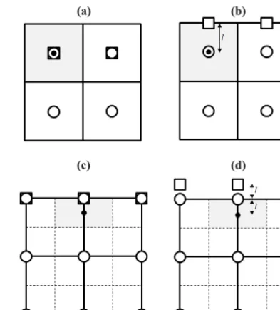
The common node approach defines a head continuity be-tween the topmost subsurface nodes and the surface nodes. This continuity requires that the topmost subsurface nodes and the surface nodes are colocated at the land surface such that there is a continuity in the elevation head. This require-ment is automatically fulfilled in vertex-centered schemes. Figure 1a illustrates the configuration of common nodes in ParFlow, a cell-centered scheme (R. Maxwell, personal com-munication in relation to previous work of the author, 2011; de Rooij et al., 2013a). Figure 1c illustrates the configuration of common nodes for vertex-centered schemes. This con-figuration is similar to the concon-figuration used in HydroGeo-Sphere (Therrien et al., 2010).

Considering that nodal values ideally represent the mean values within discrete control volumes, as described in Sect. 2, it can be argued that the head continuity as imple-mented in the common node approach is not in agreement with the physical principle of head continuity at the land sur-face. Namely, the common node approach enforces a conti-nuity between surface heads at the land surface and the mean subsurface heads within the topmost subsurface discrete con-trol volumes which have a finite thickness. This is different from enforcing a continuity between surface heads and sub-surface heads within an infinitesimally thin subsub-surface layer directly below the land surface. As such, the common node approach is only numerically correct if the topmost subsur-face cells are very thin.

4 Dual node approach 4.1 Basics

Figure 1b and c illustrate the classical arrangement of surface and subsurface nodes in cell-centered and vertex-centered fi-nite difference schemes, respectively. Commonly, the dual node approach is expressed in terms of an exchange fluxqe (L T−1) computed as follows (Liggett et al., 2012; Panday and Huyakorn, 2004):

qe=fpKz

l (hs−hss) , (1)

Figure 1. (a)Common nodes in cell-centered schemes. (b)Dual nodes in cell-centered schemes.(c)Common nodes and colocated dual nodes in vertex-centered schemes.(d)Dual nodes in vertex-centered schemes (not colocated). The white squares and white cir-cles represent surface and subsurface nodes, respectively. The solid and dashed lines represent the primary mesh and the dual mesh, respectively. The grey-shaded area is a topmost discrete volume as-sociated with a topmost subsurface node. The black dot represents the centroid of this volume. The coupling lengthlas depicted in this figure applies to the consistent dual node approach.

wherehsandhssare the hydraulic heads (L) associated with the surface node and the topmost subsurface node, respec-tively,fp(–) is the fraction of the interface that is ponded and lis the coupling length (L). The ponded fraction of the inter-face is typically defined by a function that varies smoothly between zero at the land surface elevation and unity at the rill storage height which defines the minimum water depth for initiating lateral overland flow (Panday and Huyakorn, 2004). In Eq. (1) the termfpKz/ lis commonly referred to as

the first-order exchange parameter, where first-order means that the exchange flux depends linearly on the hydraulic head difference.

4.2 Consistent dual node approach

In the following, it is illustrated that the dual node approach can and should be derived from basic equations that describe infiltration into a porous medium. Using Darcy’s law, the in-filtration rate at the ponded land surfaceqs→ss(L T−1) can be written as a function of the vertical subsurface hydraulic gradient at the land surface:

qs→ss=

krKz

∂h ∂z

_z=z

s =Kz

∂h ∂z

_z=z

s

, (2)

where h the hydraulic head (L), z the elevation head (L), kr the relative hydraulic conductivity (–) Kz the saturated

vertical hydraulic conductivity (L T−1) andzs the elevation head at the land surface. The relative hydraulic conductivity is unity because Eq. (2) applies to the ponded land surface which implies fully saturated conditions at the land surface (i.e., ponding meansps> 0, wherepsis the pressure head at the surface). Similarly, the infiltrability (L T−1_{), defined as} the infiltration rate under the condition of atmospheric pres-sure (Hillel, 1982), can be written as follows:

I =

krKz

∂h

∂z

z=zs,ps=0 =Kz

∂h

∂z

z=zs

. (3)

The relative hydraulic conductivity is again unity because the saturation equals unity under atmospheric conditions (ps= 0). The infiltration rate at nonponded land surface qatm→ss (L T−1) can be expressed as follows:

qatm→ss=min(max(I,0) , qR) , (4)

whereqRis the effective rainfall rate (i.e., the infiltration rate is limited by either the infiltrability or the available effec-tive rainfall rate). The total exchange flux across the surface– subsurface interface can now be written as follows:

qe=fpqs→ss+ 1−fpqatm→ss. (5)

To approximate the vertical subsurface hydraulic gradient in Eqs. (2) and (3), it is crucial to recognize that, according to the principle of head continuity at the land surface, the sur-face hydraulic head at a sursur-face node must also represent the subsurface head at the land surface at that location. More-over, since the subsurface hydraulic heads at the topmost sub-surface nodes are ideally associated with the centroids of the topmost subsurface discrete control volumes, these head val-ues do not represent valval-ues at the land surface but at some depth below the land surface. Because the subsurface hy-draulic heads at the dual nodes can be and should be asso-ciated with a different elevation, the vertical subsurface head gradient between the dual nodes can be approximated by a standard finite difference approximation. If this approxima-tion is being used to approximate the gradient at the land sur-face in Eqs. (2) and (3), then this approximation is by defini-tion a one-sided first-order finite difference. By defining the

coupling length byl=1zdn, where1zdnis the difference in the mean elevation head associated with the dual nodes, the infiltration rate and infiltrability can thus be computed with the following one-sided finite difference approximation:

Kz

∂h ∂z

z=zs ≈Kz

l (hs−hss) . (6)

The above definition of the coupling lengthl=1zdnensures a proper approximation of the vertical gradient in elevation head at the land surface:

∂z ∂z

z=zs

=1zdn

l =1. (7)

The above derivation of the consistent dual node approach from basic flow equations has implications for how the dual node approach is conceptualized and how it should be imple-mented. The idea that the coupling length must be directly related to the spatial discretization is an important new in-sight. Namely, as the coupling length is related to grid topol-ogy, it does not represent a nonphysical parameter associ-ated with a distinct interface separating the two domains. It is also crucial to observe the difference between the consis-tent dual node approach and the common node approach re-garding how the head continuity at the surface–subsurface interface is formulated. As explained in Sect. 2, the formu-lation in the common node approach is only correct if the topmost subsurface discrete volumes are very thin. In com-parison, the formulation in the dual node approach is correct irrespective of the vertical discretization. Namely, irrespec-tive of the vertical discretization the surface hydraulic heads equal the subsurface heads at the interface.

Yu (2014) and Kumar et al. (2009) are actually quite different from the common node approach. As already mentioned, the consistent dual node scheme differs from the common node approach with respect to how the head continuity is formu-lated at the surface–subsurface interface. As discussed later on, this difference has crucial consequences in terms of ac-curacy as well as numerical efficiency.

In vertex-centered schemes the commonly used nodal con-figuration near the surface is such that zs=zss. However, even though the topmost subsurface node is located at the land surface in a vertex-centered scheme, the elevation head at this node should ideally correspond to the mean elevation head within the topmost subsurface discrete volume. This suggests that the topmost subsurface node should be moved to the centroid of the topmost subsurface discrete volume. Although this is a possible solution, the drawback of this solution is that the subsurface model ceases to be a purely vertex-centered scheme. Moreover, such an operation cannot be performed in finite element schemes since the nodal po-sitions define the geometry of the elements. Therefore, an alternative solution is proposed. Namely, in vertex-centered schemes the elevation of the surface nodes are changed ac-cording tozs=zss+l, wherelis equal to half the thickness of the topmost subsurface dual cell. The resulting nodal config-uration is illustrated in Fig. 1d. When applying this solution, all the topmost subsurface cells must have the same thick-ness, such that the topography is increased with the same value everywhere. In essence, the motivation behind this so-lution is that a more accurate approximation of the hydraulic gradient (i.e., enforcing a unit gradient in elevation head) is more important than the actual elevation of the land surface. Similar to the nodal configuration in ParFlow, the resulting nodal configuration may not seem ideal. Namely, the surface elevation does not coincide with the top of the subsurface grid. Nonetheless, as illustrated later on, simulation results obtained with the resulting scheme are reasonable.

To illustrate that the presented dual node approach ex-hibits consistent behavior, the necessary conditions for pond-ing due to excess infiltration and exfiltration are considered. In general, ponding starts when qR>I (Hillel, 1982). Ob-serving that Eq. (6) defines the computed infiltrability when ps=0 and that the gradient in elevation head between the dual nodes is unity, the infiltrability can be expressed by

I =Kz(1−pss/ l). Therefore,qR>Iimplies that

pss> l

1−qR

Kz

. (8)

Ponding due to excess infiltration occurs if qR/Kz>1 and

implies that saturation in the subsurface starts from the top down (Hillel, 1982). Using qR/Kz>1, it follows from

Eq. (8) thatpss is still negative at the moment of ponding. This is reasonable, because the pressure head value at the topmost subsurface node represents a value at a certain depth below the land surface. Top-down saturation implies that sat-uration at the topmost subsurface node occurs after

pond-ing and thus a negative pressure head value at this node at the moment that ponding starts. It is noted that if the ratio qR/Kzis greater than but close to unity or if the coupling

length is very small, then this condition becomespss≈0. Once ponding starts the total flux rate between the dual nodes equalsKz((ps−pss) / l+1). Top-down saturation re-quires that this flux exceeds the vertical hydraulic conductiv-ity. Reaching saturation at the topmost node (pss=0) there-fore requiresps≥0. Thus, whilepssis still negative at the moment that ponding starts, saturation at the topmost subsur-face node will occur some time after ponding started. Pond-ing due to excess saturation occurs ifqR/Kz<1 and implies

that saturation in the subsurface starts from the bottom up (Hillel, 1982). It follows from Eq. (8) that ponding due to excess saturation occurs whilepss>0. Thus, ponding starts after reaching fully saturated conditions at the topmost sub-surface node, which is again reasonable. It is noted that if the ratioqR/Kz is smaller than but close to unity or if the

cou-pling length is very small, then ponding occurs whenpss≈0.

4.3 Comparison to alternative coupling approaches To illustrate that it is crucial to account for the meaning of the values at the topmost subsurface nodes, it is instructive to consider what happens if these values are not taken as the mean values within discrete control volumes. As a first exam-ple, consider vertex-centered schemes where the dual nodes are defined such thatzss=zs, as illustrated in Fig. 1c. This is inconsistent because it defines a zero gradient in eleva-tion head between the dual nodes. Since the vertical gradi-ent in elevation head between the dual nodes is zero, the to-tal flux rate after ponding now equalsKz(ps−pss) / l.

Top-down saturation requires that this flux exceeds the vertical hydraulic conductivity. Thus, reaching saturation at the top-most subsurface node (pss=0)requires ps> l. Therefore, top-down saturation will not occur if runoff occurs and if the surface water depths remain smaller than the chosen coupling length. Indeed, it has been pointed out in other studies that the coupling length should be smaller than the rill storage height (Delfs et al., 2009; Liggett et al., 2012). The zero ver-tical gradient in elevation head between the dual nodal also means that the ponding occurs whenpss>−lqR/Kz. This

implies that ponding due to excess saturation occurs while the topmost subsurface node is not yet saturated. This dual node approach has been compared to the common node ap-proach in vertex-centered schemes (Liggett et al., 2012).

the topmost node is associated with a location at the land surface and not with the centroid of a discrete control vol-ume. This has undesirable consequences. Namely, saturating the topmost subsurface node (pss=l)due to excess infiltra-tion requires thatps> l. Indeed, when simulating excess in-filtration with MODHMS, a very small coupling length is needed to simulate top-down saturation due to excess infil-tration (Gaukroger and Werner, 2011; Liggett et al., 2013). It can also be shown that ponding due to excess saturation occurs whilepss>0. But, because of the adapted pressure– saturation relationship this means that ponding starts while the topmost subsurface node is not yet saturated. This dual node approach has been compared to the common node ap-proach in cell-centered schemes (Liggett et al., 2013).

The two comparison studies of Liggett et al. (2012, 2013) indicate that the dual node approach is typically only com-petitive with the common node approach in terms of accuracy once the coupling length is very small. However, the require-ment for a very small coupling length, is a logical conse-quence if the topmost subsurface nodal values are not taken as the mean values within discrete volumes. In essence, by choosing a very small coupling length this inconsistency is minimized. This contrasts with the consistent dual approach in which decreasing the coupling length for a given vertical discretization will result in more inaccurate simulation re-sults as this would be numerically incorrect.

CATHY (Camporese et al., 2010) as well as the model of Morita and Yen (2002) are examples of models which are neither based on the common node approach, nor a dual node approach. Both these models are conjunctive models in which the surface and subsurface flow are computed sepa-rately in a sequential fashion and in which coupling is estab-lished by matching the flow conditions along the surface– subsurface interface. A complete discussion is outside the scope of this paper, but it is worthwhile to mention that these models share some crucial characteristics with the consis-tent dual node approach. Although the two models are differ-ent, both models switch between appropriate boundary con-ditions along the surface–subsurface interface, such that in-filtration fluxes are limited to the infiltrability. In both mod-els the infiltration fluxes are computed while accounting for the unit vertical gradient in elevation head near the surface– subsurface interface. In addition, in both models ponding oc-curs when the infiltrability is exceeded.

5 Numerical experiments 5.1 Numerical model

To compare the consistent dual node approach with re-spect to the common node approach in terms of accuracy and computational efficiency numerical experiments are pre-sented. These experiments are carried out with the model code DisCo. This model code can simulate coupled surface–

subsurface flow with the dual node approach using a fully implicit or monolithic scheme (de Rooij et al., 2013b). Sub-surface flow is governed by the Richards’ equation while sur-face flow is governed by the diffusive wave equation.

Starting from a dual node scheme, the implementation of a common node scheme is relatively straightforward. If the surface nodes are numbered last, a permutation vector can be constructed which gives the corresponding topmost sub-surface node for each sub-surface node. Then, the node number-ing used in the original dual node scheme can still be used to compute the surface and subsurface flow terms. Subse-quently, using the permutation vector, the surface and sub-surface flow terms associated with a common node can be combined into the same row of the global matrix system. In addition, when using the common node approach, there is no need to evaluate exchange flow terms between the two flow domains. It is noted that the surface flow and subsurface flow computations are exactly the same irrespective of the coupling approach. As such, the model permits comparison between the two approaches in terms of accuracy as well as numerical efficiency.

An adaptive error-controlled predictor–corrector one-step Newton scheme (Diersch and Perrochet, 1999) is used in which a single user-specified parameter controls the con-vergence as well the time stepping regime. Although this scheme may not be necessary the most efficient scheme, it ensures that the time discretization error is the same irrespec-tive of the applied coupling approach. For brevity, further de-tails about the model are not discussed here and can be found elsewhere (de Rooij et al., 2013b).

5.2 Hillslope scenarios

The model code is applied to a set of three hillslope sce-narios. Table 1 lists the abbreviations used in the figures to distinguish between the coupling approaches, and to dis-tinguish between cell-centered and vertex-centered schemes. Each scenario is solved using different but uniform vertical discretizations, and1zspecifies the discretization of the pri-mary grid. The first two simulation scenarios consider hill-slope problems as designed by Sulis et al. (2010). For the purpose of this study, a third scenario is considered in which the initial and boundary conditions are different in order to create a flooding wave across an unsaturated hillslope. The problems consist of a land surface with a slope of 0.05 which is underlain by a porous medium. The domain is 400 m long and 80 m wide. The subsurface is 5 m thick. In the direction of the length and in the direction of the width, the discretiza-tion is 80 m. Different vertical discretizadiscretiza-tions are consid-ered. The van Genuchten parameters are given bysr=0.2,

ss =1.0,α=1 m−1 andn=2. The porosity is 0.4 and the

ef-Time [min]

Ru

no

ff

[

m

min

-1

]

3

0 100 200 300

0 2 4 6 8 10

dn(cc) z = 0.0125 m cn(cc) z = 0.0125 m dn(vc) z = 0.0125 m cn(vc) z = 0.0125 m

(a)

Time [min]

Runoff

[m

3

min

]

0 100 200 300

0 2 4 6 8 10

dn(cc) z = 0.0125 m dn(cc) z = 0.2 m cn(cc) z = 0.2 m dn(vc) z = 0.2 m cn(vc) z = 0.2 m

(b)

Figure 2.Outflow response for excess saturation on a hillslope (first scenario) using different vertical discretizations.

Time [min]

Ne

wt

on

st

ep

s

0 100 200 300

0 200 400 600 800

dn(cc) z = 0.0125 m cn(cc) z = 0.0125 m dn(vc) z = 0.0125 m cn(vc) z = 0.0125 m

(a)

Time [min]

Ne

wt

on

st

ep

s

0 100 200 300

0 200 400 600 800

dn(cc) z = 0.2 m cn(cc) z = 0.2 m dn(vc) z = 0.2 m cn(vc) z = 0.2 m

(b)

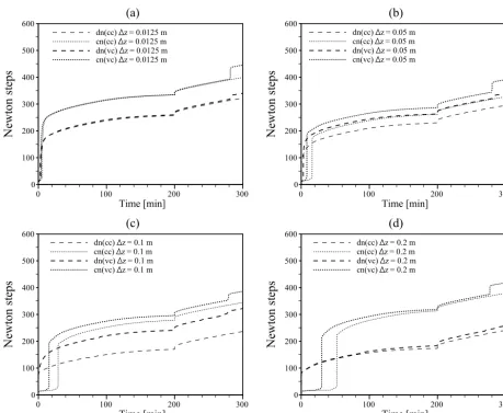
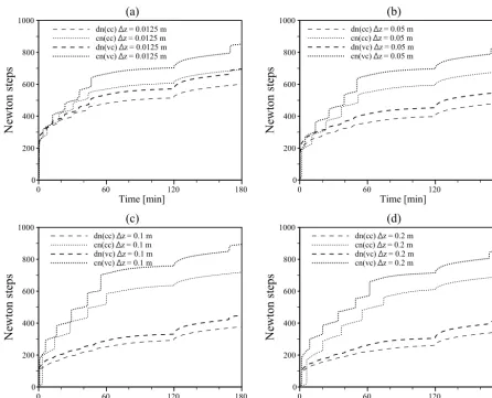
Figure 3.Number of Newton steps for excess saturation on a hillslope (first scenario) using different vertical discretizations.

Table 1.Abbreviations used in the figures.

Abbreviation Meaning

cc cell-centered

vc vertex-centered

dn dual node

cn common node

fective rainfall rate of 3.3×10−4_{m min}−1_{for a duration of} 200 min and the initial water table depth is at a depth of 1.0 m below the land surface.

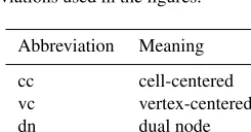
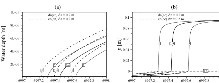
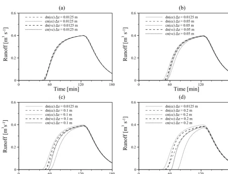
The first scenario considers excess saturation, and the sat-urated conductivity equals 6.94×10−4m min−1. Figures 2 and 3 illustrate the simulated runoff and the number of New-ton steps, respectively. Figures 4 and 5 illustrate the subsur-face pressure heads at the topmost subsursubsur-face nodes and the water depths on the surface nodes. For the second scenario,

Time [s]

Wa

te

r

de

pt

h

[m

]

7027.6 7027.8 7028 7028.2 7028.4

2E-06 4E-06 6E-06 8E-06 1E-05

dn(cc) z = 0.0125 m cn(cn) z = 0.0125 m

(a)

5 2-4 1

Time [s]

p

[m

]

7027.6 7027.8 7028 7028.2 7028.4

-0.01 -0.005 0 0.005 0.01

dn(cc) z = 0.0125 m cn(cc) z = 0.0125 m

(b)

1 2-4 5

Figure 4. Simulated values at the common nodes for excess saturation on a hillslope (first scenario) with a cell-centered scheme and

1z=0.0125 m.(a)Water depths.(b)Pressure heads. Nodes are numbered 1–5 in the downslope direction.

Time [s]

Wa

te

r

de

pt

h

[m

]

6997 6997.2 6997.4 6997.6 6997.8 6998

2E-06 4E-06 6E-06 8E-06 1E-05

dn(cc) z = 0.2 m cn(cn) z = 0.2 m

(a)

5 2-4 1

5 2-4 1

Time [s]

p

[m

]

6997 6997.2 6997.4 6997.6 6997.8 6998

0 0.02 0.04 0.06 0.08

0.1 dn(cc) z = 0.2 m_{cn(cc) z = 0.2 m}

(b)

1 2-4 5

1-5

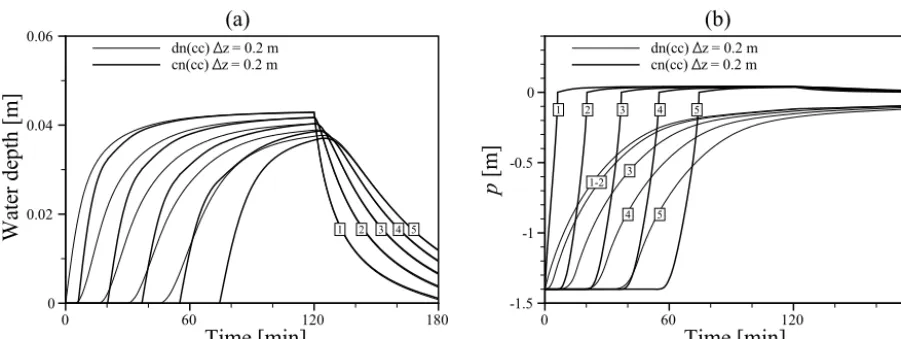
Figure 5.Simulated values for excess saturation on a hillslope (first scenario) with a cell-centered scheme and1z=0.2 m.(a)Water depths at the surface nodes.(b)Pressure heads at the topmost subsurface nodes. Nodes are numbered 1–5 in the downslope direction.

nodes for the finest and the coarsest vertical discretization, respectively.

6 Discussion 6.1 Accuracy

As discussed by Ebel et al. (2009) and confirmed by oth-ers (Liggett et al., 2012) the dual node approach mimics the common node approach if the coupling length becomes suffi-ciently small. When comparing the consistent dual node ap-proach and the common node apap-proach a very similar ob-servation applies. If the topmost subsurface cells are very thin, then the coupling length in the consistent dual node ap-proach is very small. Also, if the topmost subsurface cells are sufficiently thin then the formulation of head continu-ity at the surface–subsurface interface in the common node

approach is correct. Thus, the common node approach will mimic the consistent dual node approach. Indeed, the simu-lation results indicate that a relatively fine vertical discretiza-tion yields similar results for the common node approach as well as for the consistent dual node approach (Figs. 2a, 4a, 6a, 8a, 10a and 12a).

Time [min]

Runoff

[m

3

min

]

0 100 200 300

0 2 4 6 8 10 12 14

dn(cc) z = 0.0125 m dn(cc) z = 0.05 m cn(cc) z = 0.05 m dn(vc) z = 0.05 m cn(vc) z = 0.05 m

(b)

Time [min]

Ru

no

ff

[

m

min

-1

]

3

0 100 200 300

0 2 4 6 8 10 12 14

dn(cc) z = 0.0125 m dn(cc) z = 0.1 m cn(cc) z = 0.1 m dn(vc) z = 0.1 m cn(vc) z = 0.1 m

(c)

Time [min]

Runoff

[m

3

min

]

0 100 200 300

0 2 4 6 8 10 12 14

dn(cc) z = 0.0125 m dn(cc) z = 0.2 m cn(cc) z = 0.2 m dn(vc) z = 0.2 m cn(vc) z = 0.2 m

(d)

Time [min]

Runoff

[m

3

min

-1

]

0 100 200 300

0 2 4 6 8 10 12 14

dn(cc) z = 0.0125 m cn(cc) z = 0.0125 m dn(vc) z = 0.0125 m cn(vc) z = 0.0125 m

(a)

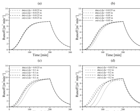
Figure 6.Outflow response for excess infiltration on a hillslope (second scenario) using different vertical discretizations.

6.1.1 Excess saturation

The simulation results of runoff due to excess saturation, as obtained by the common node approach and the consistent dual node approach as depicted in Fig. 2, illustrate that simu-lating excess saturation runoff is not significantly affected by the vertical discretization. This is because the time needed to reach fully saturated conditions in the subsurface is a simple function of the flow boundary conditions and the initial wa-ter content. It is thus expected that the vertical discretization does not significantly affect the simulation of excess satura-tion. Although the vertical discretization may affect the com-puted initial water content, this effect is usually negligible. It has been found in other studies that the vertical discretization has little effect on simulated runoff due to excess saturation (Kollet and Maxwell, 2006; Sulis et al., 2010).

6.1.2 Excess infiltration

When simulating excess infiltration the common node ap-proach requires fully saturated conditions at the topmost sub-surface node for ponding to occur. However, top-down

satu-ration associated with excess infiltsatu-ration implies that reach-ing fully saturated conditions in the topmost subsurface dis-crete volumes should require more time than reaching fully saturated conditions at the land surface, especially if the ver-tical discretization is relatively coarse. It is thus expected that the common node approach delays runoff and that this delay increases for a coarser vertical discretization. In addi-tion, if the saturation fronts are less sharp due to a relatively coarse vertical discretization, it takes more time to reach sat-urated conditions at the common node. This will further de-lay runoff. Indeed, the simulation results indicate clearly that runoff is delayed when using the common node approach, particularly if the vertical discretization is relatively coarse (Figs. 6, 9a, 10 and 13a). It has also been found in other studies that the common node approach delays runoff due to excess infiltration if the vertical discretization is relatively coarse (Sulis et al., 2010).

in-Ne

wt

on

st

ep

s

0 100 200 300

0 100 200 300 400 500 600

dn(cc) z = 0.05 m cn(cc) z = 0.05 m dn(vc) z = 0.05 m cn(vc) z = 0.05 m

(b)

Time [min]

Ne

wt

on

st

ep

s

0 100 200 300

0 100 200 300 400 500 600

dn(cc) z = 0.1 m cn(cc) z = 0.1 m dn(vc) z = 0.1 m cn(vc) z = 0.1 m

(c)

Time [min]

Ne

wt

on

st

ep

s

0 100 200 300

0 100 200 300 400 500 600

dn(cc) z = 0.2 m cn(cc) z = 0.2 m dn(vc) z = 0.2 m cn(vc) z = 0.2 m

(d)

Time [min]

Ne

wt

on

st

ep

s

0 100 200 300

0 100 200 300 400 500 600

dn(cc) z = 0.0125 m cn(cc) z = 0.0125 m dn(vc) z = 0.0125 m cn(vc) z = 0.0125 m

(a)

Time [min]

Figure 7.The total number of Newton steps for excess infiltration (second scenario) on a hillslope using different vertical discretizations.

Time [min]

Wa

te

r

de

pt

h

[m

]

0 60 120 180 240 300

0 0.01 0.02 0.03

dn(cc) z = 0.0125 m cn(cc) z = 0.0125 m

(a)

5

3 4

2

1

Time [min]

p

[m

]

0 60 120 180 240 300

-0.2 -0.15 -0.1 -0.05 0 0.05 0.1

dn(cc) z = 0.0125 m cn(cc) z = 0.0125 m

(b)

1-5 1-5

Figure 8.Simulated values at the common nodes for excess infiltration on a hillslope (second scenario) with a cell-centered scheme and

Time [min]

Wa

te

r

de

pt

h

[m

]

0 60 120 180 240 300

0 0.01 0.02 0.03

dn(cc) z = 0.2 m cn(cc) z = 0.2 m

(a)

5

3 4

2

1

Time [min]

p

[m

]

0 60 120 180 240 300

-1 -0.8 -0.6 -0.4 -0.2 0 0.2

dn(cc) z = 0.2 m cn(cc) z = 0.2 m

(b)

1-5 1-5

Figure 9.Simulated values for excess infiltration on a hillslope with a cell-centered scheme (second scenario) and1z=0.2 m.(a)Water depths at the surface nodes.(b)Pressure heads at the topmost subsurface nodes. Nodes are numbered 1–5 in the downslope direction.

R

unoff

[m

3

s

-1

]

0 60 120 180

0 0.2 0.4 0.6

dn(cc) z = 0.0125 m dn(cc) z = 0.05 m cn(cc) z = 0.05 m dn(vc) z = 0.05 m cn(vc) z = 0.05 m

(b)

Time [min]

R

unoff

[m

s

-1

]

3

0 60 120 180

0 0.2 0.4 0.6

dn(cc) z = 0.0125 m dn(cc) z = 0.1 m cn(cc) z = 0.1 m dn(vc) z = 0.1 m cn(vc) z = 0.1 m

(c)

Time [min]

R

unoff

[m

3

s

-1

]

0 60 120 180

0 0.2 0.4 0.6

dn(cc) z = 0.0125 m dn(cc) z = 0.2 m cn(cc) z = 0.2 m dn(vc) z = 0.2 m cn(vc) z = 0.2 m

(d)

Time [min]

R

unoff

[m

3

s

-1

]

0 60 120 180

0 0.2 0.4 0.6

dn(cc) z = 0.0125 m cn(cc) z = 0.0125 m dn(vc) z = 0.0125 m cn(vc) z = 0.0125 m

(a)

Time [min]

Figure 10.Outflow response for flooding an unsaturated hillslope using different vertical discretizations.

filtrability is exceeded. Compared to the condition for pond-ing in the common node approach, this is arguably more cor-rect. Namely, if saturation occurs from the top-down then the saturation at a certain depth occurs later than saturation at the

indi-Ne

wt

on

st

ep

s

0 60 120 180

0 200 400 600 800 1000

dn(cc) z = 0.0125 m cn(cc) z = 0.0125 m dn(vc) z = 0.0125 m cn(vc) z = 0.0125 m

(a)

Time [min]

Ne

wt

on

st

ep

s

0 60 120 180

0 200 400 600 800 1000

dn(cc) z = 0.1 m cn(cc) z = 0.1 m dn(vc) z = 0.1 m cn(vc) z = 0.1 m

(c)

Time [min]

Ne

wt

on

st

ep

s

0 60 120 180

0 200 400 600 800 1000

dn(cc) z = 0.2 m cn(cc) z = 0.2 m dn(vc) z = 0.2 m cn(vc) z = 0.2 m

(d)

Time [min]

Ne

wt

on

st

ep

s

0 60 120 180

0 200 400 600 800 1000

dn(cc) z = 0.05 m cn(cc) z = 0.05 m dn(vc) z = 0.05 m cn(vc) z = 0.05 m

(b)

Time [min]

Figure 11.Number of Newton steps for flooding an unsaturated hillslope using different vertical discretizations.

Time [min]

Wa

te

r

de

pt

h

[m

]

60 120 180

0 0.02 0.04

dn(cc) z = 0.0125 m cn(cc) z = 0.0125 m

(a)

5 3 4 2 1

Time [min]

p

[m

]

0 60 120 180

-0.2 -0.15 -0.1 -0.05 0 0.05 0.1

dn(cc) z = 0.0125 m cn(cc) z = 0.0125 m

(b)

5 4 3 2

Time [min]

Wa

te

r

de

pt

h

[m

]

0 60 120 180

0 0.02 0.04 0.06

dn(cc) z = 0.2 m cn(cc) z = 0.2 m

(a)

5 3 4 2 1

Time [min]

p

[m

]

0 60 120 180

-1.5 -1 -0.5 0

dn(cc) z = 0.2 m cn(cc) z = 0.2 m

(b)

5 5

4 1-2

4 3 2 1

3

Figure 13.Simulated values for excess infiltration (third scenario) on a hillslope with a cell-centered scheme and1z=0.2 m.(a)Water depths at the surface nodes.(b)Pressure heads at the topmost subsurface nodes. Nodes are numbered 1–5 in the downslope direction.

cated in Figs. 6b–d, 9a, 10b–d and 13a. To further explain this difference in accuracy, it is emphasized that the spatial resolution only affects the accuracy of the flow computations when using the consistent dual node approach and that the formulation of head continuity at the interface remains cor-rect. In contrast, when using the common node approach, if the spatial resolution is too coarse then this does not only affect the accuracy of the flow computations but in addition the formulation of head continuity becomes incorrect. It must be emphasized, however, that regardless of the applied cou-pling approach, the vertical discretization must be relatively fine. As indicated by Figs. 6b–d, 9a, 10b–d and 13a the dif-ference between the simulated results and the redif-ference so-lution increases for a coarser discretization. Eventually such differences will lead to unreasonable results regardless of the coupling approach.

It is interesting to note that An and Yu (2014) also found that their model was less sensitive to the vertical discretiza-tion in comparison to ParFlow when simulating runoff due to excess infiltration. Whereas An and Yu (2014) hypothesized that this difference in performance was related to using ir-regular grids instead of orthogonal grids as in ParFlow, it is argued here that this difference can be explained by the fact that both models use a different coupling approach.

Although the consistent dual node approach is less sensi-tive to the vertical discretization in comparison to the com-mon node approach, it is useful to explain in detail how the vertical discretization affects the accuracy of the consistent dual node approach to the vertical discretization. A relatively coarse vertical discretization may result in an underestima-tion of the vertical pressure gradient at the land surface. This is because, in a soil close to hydrostatic conditions, the pres-sure heads increase with depth. Therefore, the infiltrability during the early stages of infiltration may be underestimated. If the applied flux rate is sufficiently large such that the un-derestimated infiltrability is exceeded, then runoff during the

early stages will be overestimated. Figure 6d illustrates that runoff is indeed overestimated at early times when simulated with the cell-centered scheme, a relatively coarse vertical dis-cretization and a consistent dual node approach. During the later stages of infiltration the pressure head at the topmost subsurface node will be underestimated due to the combined effect of an underestimated infiltration rate and the overly diffused saturation fronts. This results in an overestimation of the infiltration rate in the later stages. Thus, at some time after ponding has started, it is expected that the amount of runoff is underestimated.

If the underestimated infiltrability is not exceeded, then the overly diffused saturation fronts resulting from a relatively coarse vertical discretization will eventually lead to an under-estimation of pressure head at the topmost subsurface node, and as such the infiltrability may be overestimated at later times. Consequently, when using the consistent dual node approach, runoff due to excess infiltration may be delayed. However, the delay in runoff as simulated by the consistent dual node approach will only equal the delay in runoff as simulated by the common node approach in the limit when qR/Kz goes to unity. Namely, as explained in Sect. 4.2, if

qR/Kzgoes to unity, then the consistent dual node approach

behaves similarly to a common node approach. However, in general, if the consistent dual node approach delays runoff, this delay will be smaller than the delay in runoff as simu-lated by the common node approach.

ad-vances downstream for relatively fine as well as relatively coarse vertical discretizations, as depicted in Fig. 13a.

As illustrated in Figs. 6b–d and 10b–d, if the coupling ap-proach and the vertical discretization are identical, then the vertex-centered schemes are closer to the reference solution with respect to the cell-centered schemes. This difference re-sults solely from the fact that the primary mesh is the same for both schemes. As such, the vertical extent of the topmost subsurface volumes is twice as small when using the vertex-centered scheme. This difference in vertical grid resolution near the land surface explains the differences between the schemes.

6.2 Computational efficiency

The computational efficiency of the schemes is measured in terms of the number of Newton steps. The number of Newton steps equals the number of times that the linearized system of equations is solved, and this number depends on the time step sizes as well as the number of failed Newton steps. It is emphasized that the measured efficiency depends crucially on the applied model code. Nonetheless, as shown in the fol-lowing, the measured differences in efficiencies can be ex-plained in terms of abrupt changes in how fast pressure heads near the surface–subsurface interface are evolving with time. Regardless of the type of scheme used to solve the nonlinear flow equations, such abrupt changes are difficult to solve.

Once ponding occurs a surface–subsurface flow model will encounter significant numerical difficulties as surface flow terms are activated. In essence, the activation of these terms represents a discontinuity in flow behavior which is challenging to resolve (Osei-Kuffuor et al., 2014). Indeed, the Newton steps as depicted in Figs. 3 and 7 indicate that simulations encounter difficulties at the moment of ponding. These figures also indicate that the consistent dual node ap-proach can be more efficient in comparison to the common node approach.

6.2.1 Excess saturation

Just before the moment of ponding due to excess saturation, the rate of change in pressure heads at the topmost subsurface nodes is relatively high for both coupling approaches. This high rate is related to the shape of the water retention curve. Typically, the derivative of the saturation with respect to the pressure head goes to zero when approaching fully saturated conditions. Once ponding starts, the surface flow terms are activated and therefore the rate of change in pressure heads at the topmost subsurface nodes decreases drastically. Both approaches must handle this drastic change. However, from Figs. 4b and 5b it can be observed that the rate of change decreases more abruptly when using the common node ap-proach.

When using the common node approach the vertical hy-draulic gradients in the subsurface are close to zero at the

moment of ponding, since additional water volumes can only be accommodated by means of specific storage. This implies that the infiltration rate drops instantaneously at the moment of ponding. In contrast, in the dual node approach, ponding starts when the infiltrability is exceeded. Thus, at the mo-ment of ponding, the infiltration rate is higher in comparison to the common node approach. After ponding this infiltra-tion rate will decrease quickly as the hydraulic heads at the dual nodes equilibrate. This difference in the infiltration rate at the moment of ponding explains why the topmost subsur-face hydraulic heads change more smoothly when using the dual node approach. If the vertical discretization is coarser, then the infiltration rate at the moment of ponding, computed with the consistent dual node approach, is even higher and this results in a lower initial rate initial rate of change in wa-ter depth, as depicted in Fig. 5a.

The more abrupt changes in pressure heads at the com-mon node in comparison to the changes in pressure heads at the dual nodes mean that solving the activation of pond-ing with the common node approach is more difficult. It is noted that the differences in the infiltration rates between the two coupling approaches only occur at the moment of pond-ing and directly thereafter when water depths are relatively small. Namely, quickly after ponding, the hydraulic heads at the dual nodes will equilibrate and after that the two coupling approaches will behave similar. This explains why these dif-ferences in infiltration rates do not significantly affect the ac-curacy of simulated runoff.

6.2.2 Excess infiltration

Figures 7 and 11 also indicate that a coarser vertical dis-cretization only provides a significant gain in efficiency in terms of Newton steps when using the consistent dual node approach. When using the common node approach, a coarser discretization does not change the fact that the topmost sub-surface node must reach fully saturated conditions for pond-ing to occur and that the infiltration rate is relatively high just before ponding. When using the consistent dual node approach, a coarser vertical discretization means that the sat-uration fronts are more diffused such that the flow problem becomes easier to solve.

Figure 8a and 9a illustrate that for the second simulation scenario, ponding occurs almost simultaneously at all the surface nodes. Figure 12a and 13a show that this is different for the third scenario where ponding occurs at different times as the flooding wave travels downstream. When Fig. 11a is compared with Fig. 12a and when Fig. 11d is compared with Fig. 13a, it is clear that the common node approach encoun-ters difficulties around each time ponding starts at a surface node. Figure 11 shows that these difficulties are encountered for all discretizations. In contrast the consistent dual node ap-proach has much fewer difficulties solving these problems. As discussed in Sect. 6.1.2, the common node approach may result in steepening the advancing wave. This implies that water depths will be changing more quickly. This presents an additional difficulty for solving this flow problem with the common node approach.

7 Conclusions

In this study it is shown that the dual node approach should be conceptualized and implemented as a one-sided finite dif-ference approximation of the vertical hydraulic gradient at the land surface. This provides an important new insight into the coupling length. Namely, if the dual node approach is properly implemented then the coupling length is related to the vertical grid resolution. Thus, the coupling length does not represent an additional nonphysical model parameter, and therefore the dual node approach is not automatically a less physically based approach in comparison to the common node approach. Actually, this study shows if the vertical dis-cretization is not sufficiently fine then the head continuity at the surface–subsurface interface is formulated more correctly in the consistent dual node scheme. This difference in formu-lation has consequences for how both approaches compare in terms of accuracy and efficiency.

Numerical experiments indicate that the consistent dual node approach is equally accurate or more accurate than the common node approach. It has been shown that in compari-son to the common node approach the consistent dual node approach is less sensitive to the vertical discretization when simulating excess infiltration. However, the practical advan-tage of the consistent dual node approach in terms of accu-racy is limited. Namely, if the vertical discretization is

re-fined, both approaches will converge to more accurate and eventually similar results when simulating excess infiltration. When simulating excess saturation, both approaches yield similar results even if the vertical discretization is relatively coarse.

Nonetheless, even though the advantage of the consistent dual node approach in terms of accuracy is limited, the fact that the consistent dual node approach is equally or more ac-curate than the common node approach is a significant find-ing. Namely, this finding is different from the commonly held view that a dual node approach is most accurate if it mim-ics the common node approach. Moreover, it also illustrates clearly that the consistent dual node approach is not similar to a common node approach.

Numerical experiments indicate that the consistent dual node approach can be more efficient than the common node approach while being equally or more accurate than the com-mon node approach. It has been shown that this difference in efficiency is related to abrupt changes in the evolution of pressure heads around the moment that ponding is initiated.

Based on the findings in this study the models of An and Yu (2014) and Kumar et al. (2009) are expected to have some advantages with respect to models that are based on the com-mon node approach. This is because these models are based on a consistent dual node approach. Moreover, given a model that uses an alternative dual node approach, it is relatively straightforward to implement the numerically more correct consistent dual node approach.

Code availability. The model code can be obtained from the author.

Competing interests. The author declares that he has no conflict of interest.

Acknowledgements. This research was funded by the Carl S. Swisher Foundation.

Edited by: Philippe Ackerer

Reviewed by: three anonymous referees

References

An, H., and Yu, S.: Finite volume integrated surface- subsurface flow modeling on nonorthogonal grids, Water Resour. Res., 50, 2312–2328, 2014.

Blazek, J.: Computational fluid dynamics: Principles and applica-tions, Elsevier, Oxford, UK, 2005.

Delfs, J. O., Park, C. H., and Kolditz, O.: A sensitivity analysis of Hortonian flow, Adv. Water Res., 32, 1386–1395, 2009. de Rooij, R., Graham, W., and Maxwell, R.: A particle-tracking

scheme for simulating pathlines in coupled surface-subsurface flows, Adv. Water Res., 52, 7–18, 2013a.

de Rooij, R., Perrochet, P., and Graham, W.: From rainfall to spring discharge: Coupling conduit flow, subsurface matrix flow and surface flow in karst systems using a discrete-continuum model, Adv. Water Res., 61, 29–41, 2013b.

Diersch, H. J. G. and Perrochet, P.: On the primary variable switch-ing technique for simulatswitch-ing unsaturated-saturated flows, Adv. Water Res., 23, 271–301, 1999.

Ebel, B. A., Mirus, B. B., Heppner, C. S., VanderKwaak, J. E., and Loague, K.: First-order exchange coefficient coupling for sim-ulating surface water-groundwater interactions: parameter sen-sitivity and consistency with a physics-based approach, Hydrol. Process., 23, 1949–1959, 2009.

Gaukroger, A. M. and Werner, A. D.: On the Panday and Huyakorn surface-subsurface hydrology test case: analysis of internal flow dynamics, Hydrol. Process., 25, 2085–2093, 2011.

Hillel, D.: Introduction to soil physics, Academic press, New York, USA, 1982.

Kolditz, O. and Shao, H.: OpenGeoSys, Developer-Benchmark-Book, OGS-DBB 5.04, Helmholtz Centre for Environmental Re-search (UFZ), Leipzig, Germany, 2010.

Kollet, S. J. and Maxwell, R. M.: Integrated surface-groundwater flow modeling: A free-surface overland flow boundary condition in a parallel groundwater flow model, Adv. Water Res., 29, 945– 958, 2006.

Kumar, M., Duffy, C. J., and Salvage, K. M.: A Second-Order Ac-curate, Finite Volume-Based, Integrated Hydrologic Modeling (FIHM) Framework for Simulation of Surface and Subsurface Flow, Vadose Zone J., 8, 873–890, 2009.

Liggett, J. E., Werner, A. D., and Simmons, C. T.: Influence of the first-order exchange coefficient on simulation of coupled surface-subsurface flow, J. Hydrol., 414, 503–515, 2012.

Liggett, J. E., Knowling, M. J., Werner, A. D., and Simmons, C. T.: On the implementation of the surface conductance approach us-ing a block-centred surface-subsurface hydrology model, J. Hy-drol., 496, 1–8, 2013.

Morita, M. and Yen, B. C.: Modeling of conjunctive two-dimensional surface-three-two-dimensional subsurface flows, J. Hy-draul. Eng.-ASCE, 128, 184–200, 2002.

Moukalled, F., Mangani, L., and Darwish, M.: The Finite Vol-ume Method in Computational Fluid Dynamics, Springer, Cham, Switzerland, 2016.

Osei-Kuffuor, D., Maxwell, R. M., and Woodward, C. S.: Improved numerical solvers for implicit coupling of subsurface and over-land flow, Adv. Water Res., 74, 185–195, 2014.

Pan, L. and Wierenga, P. J.: A transferred pressure head based ap-proach to solve Richards equation for variably saturated soils, Water Resour. Res., 31, 925–931, 1995.

Panday, S. and Huyakorn, P. S.: A fully coupled physically-based spatially-distributed model for evaluating surface/subsurface flow, Adv. Water Res., 27, 361–382, 2004.

Ross, P. J.: Efficient numerical methods for infiltration using Richards equation, Water Resour. Res., 26, 279–290, 1990. Sulis, M., Meyerhoff, S. B., Paniconi, C., Maxwell, R. M., Putti,

M., and Kollet, S. J.: A comparison of two physics-based nu-merical models for simulating surface water-groundwater inter-actions, Adv. Water Res., 33, 456–467, 2010.

Therrien, R., McLaren, R. G., Sudicky, E. A., and Panday, S. M.: HydroGeoSphere-a three-dimensional numerical model describ-ing fully-integrated subsurface and surface flow and solute trans-port (draft), Groundwater Simulations Group, University of Wa-terloo, WaWa-terloo, Canada, 2010.

VanderKwaak, J. E.: Numerical simulation of flow and chemical transport in integrated surface-subsurface hydrologic systems, University of Waterloo, Waterloo, Canada, 1999.

Yeh, G.-T., Shih, D.-S., and Cheng, J.-R. C.: An integrated media, integrated processes watershed model, Comput. Fluids, 45, 2–13, 2011.