Technical note: Uncertainty in multi source partitioning using large tracer data sets

(1)

https://doi.org/10.5194/hess-23-5059-2019 © Author(s) 2019. This work is distributed under the Creative Commons Attribution 4.0 License.

Technical note: Uncertainty in multi-source partitioning

using large tracer data sets

Alicia Correa1,2, Diego Ochoa-Tocachi3, and Christian Birkel1,4

1_{Department of Geography and Water and Global Change Observatory, University of Costa Rica, San José, 2060, Costa Rica} 2_{Institute for Applied Sustainability Research (iSUR), Quito, 170503, Ecuador}

3_{Department of Mathematics, Universidad San Francisco de Quito, Quito, 170901, Ecuador} 4_{Northern Rivers Institute, University of Aberdeen, Aberdeen, AB24 3UF, UK}

Correspondence:Alicia Correa ([email protected]) Received: 27 April 2019 – Discussion started: 21 May 2019

Revised: 25 October 2019 – Accepted: 30 October 2019 – Published: 16 December 2019

Abstract. The availability of large tracer data sets opened up the opportunity to investigate multiple source contribu-tions to a mixture. However, the source contribucontribu-tions may be uncertain and, apart from Bayesian approaches, to date there are only solid methods to estimate such uncertainties for two and three sources. We introduce an alternative uncer-tainty estimation method for four sources based on multiple tracers as input data. Taylor series approximation is used to solve the set of linear mass balance equations. We illustrate the method to compute individual uncertainties in the calcu-lation of source contributions to a mixture, with an example from hydrology, using a 14-tracer set from water sources and streamflow from a tropical, high-elevation catchment. More-over, this method has the potential to be generalized to any number of tracers across a range of disciplines.

1 Introduction

Tracer applications have dramatically increased over re-cent years across a wide range of disciplines (West et al., 2010). Applications in hydrology (Hooper, 2003; James and Roulet, 2006; Kirchner and Neal, 2013), ecology (Phillips and Gregg, 2003; Semmens et al., 2009b), anthropology (Ehleringer et al., 2008), conservation biology (Bicknell et al., 2014), nutrition (Magaña-Gallegos et al., 2018), environ-mental and ecosystem science (Bartov et al., 2013; Granek et al., 2009), and erosion and sediment transportation (Davies et al., 2018) have been the most prominent. Such widespread use of tracers was mainly facilitated by the availability of

an-alytical techniques that provide highly sensitive, rapid multi-element analysis at a lower cost (Falkner et al., 1995). For example, the use of inductively coupled plasma mass spec-trometry (ICP-MS) as one of the most relevant analytical techniques for elemental analysis (Helaluddin et al., 2016) led to the availability and use of large tracers sets (elements) in hydrological studies (Barthold et al., 2017; Belli et al., 2017; Correa et al., 2017; Kirchner and Neal, 2013; Mimba et al., 2017). Trace elements together with water stable iso-topes (cavity ringdown laser absorption spectroscopy paved the way: Berman et al., 2009; Lis et al., 2008) as well as physical–chemical water parameters (e.g. electrical conduc-tivity and pH) are now often used to improve understanding of hydro-geochemical cycles, flow pathways and runoff gen-eration in hydrology. Furthermore, mixing models based on tracer mass balance equations are widely applied to identify the dominant sources of a mixture and their contribution dy-namics.

(2)

was developed to use multiple tracers as input and, there-fore, allows for a multi-dimensional space that potentially increases the number of identifiable sources (Barthold et al., 2011; Inamdar et al., 2013; Liu et al., 2004). In addition, the use of multiple tracers can avoid bias and subjectivity in the input information. Therefore, EMMA provides a ro-bust and complete conceptualization of catchment function-ing and source interactions durfunction-ing runoff generation (Iwasaki et al., 2015). However, despite its benefits, the EMMA ap-proach lacks a formal methodology to assess the uncertainty of multiple end-members (Delsman et al., 2013) and their individual uncertainties in the calculation of source contribu-tions to a stream.

To our knowledge, the uncertainty estimation of source contributions to streams is based on Gaussian error propaga-tion (Genereux, 1998) and was so far only calculated using one or two tracers simultaneously (MixSIAR: Parnell et al., 2010; Phillips and Gregg, 2001; Semmens et al., 2009a). Al-ternatively, when the number of sources is higher, the uncer-tainty is usually based on the sum of analytical errors, eleva-tion effects and the spatial variability of end-member concen-trations (Uhlenbrook and Hoeg, 2003). Hence, we propose an alternative methodology based on the first-order Taylor series approximation to estimate the uncertainty of individ-ual end-members or sources (e.g. precipitation, soil water, groundwater) to a mixture (e.g. streamflow).

We illustrate this application using a multi-tracer data set from Correa et al. (2019b), in a three-dimensional space de-fined by a principal component analysis (PCA). In Correa et al. (2019b), the authors computed the uncertainties but with-out disclosing any details in the calculation and methodology used. The main objective of this technical note is, therefore, to explicitly describe the mathematical development that al-lows the calculation of partial derivatives, degrees of free-dom and confidence interval limits for each source fraction contribution and, moreover, to provide the code and several examples for their calculation and reproducibility.

2 Uncertainty estimation method development

In this section, the uncertainty estimation method presented in Phillips and Gregg (2001) is expanded for four source con-tributions to the mixture.

LetCrepresent the following set of sources:A,B,Cand D, and mixture M, C= {A, B, C, D, M}. In the following equations,x∈C,y∈δ, λ, φ andz∈ {A, M, C}.x,yandz are variables that belong to the following sets:xto the set of A,B,C,Dand mixtureM;yto the set of medians of every projected source and mixture in each principal component δλφ respectively of the sub index used; and zto the set of A,MandC. Furthermore,fA, fB, fC andfD represent the contribution fraction of sourcesA,B,C andDrespectively to the mixtureM.

The data required for this analysis are the median and stan-dard deviations (σ) of each of the sources (A,B,C andD) and the mixtureM, projected and expressed in the coordi-nates of the three-dimensional PCA space. As well as this, the sample size (n) of each source is required. Details of the application are presented in Sect. 3.2.

If the system is composed of Eq. (1) 

 

 

δAfA + δBfB + δCfC + δDfD = δM λAfA + λBfB + λCfC + λDfD = λM φAfA + φBfB + φCfC + φDfD = φM fA + fB + fC + fD = 1

(1)

and has solution1forfAfBfCfD>0, the contribution frac-tions take the following form:

fA=

(8M−1M) (3C−1C)−(3M−1M) (8C−1C) (8A−1A) (3C−1C)−(3A−1A) (8C−1C) =Num

Den, fC=

(1M−3M)−(1A−3A) fA (1C−3C)

, fB=1M−(1CfC+1AfA) ,

fD=1−(fC+fB+fA) , (2) where

1x=

δx−δD δB−δD

, 3x=

λx−λD λB−λD ,

8x=

φ_x−φ_D

φ_B−φ_D. (3)

The partial derivatives of Eq. (2) are given by ∂fA

∂yx

= 1

Den2

(3C−1C) _∂8

M ∂yx

−∂1M

∂yx

+(8M−1M) _∂3

C ∂yx

−∂1C

∂yx

−(8C−1C) _∂3

M ∂yx

−∂1M

∂yx

−(3M−1M) _∂8

C ∂yx

−∂1C

∂yx

Den

−

(3C−1C) _∂8

A ∂yx

−∂1A

∂yx

+(8A−1A) _∂3

C ∂yx

−∂1C

∂yx

−(8C−1C) _∂3

A ∂yx

−∂1A

∂yx

−(3A−1A) _∂8

C ∂yx

−∂1C

∂yx

Num

,

1_{The system has a solution if the vector of mixture}_M_{is on the}

polyhedron generated by the vectors of sourcesA,B,CandDsuch thatP

x

(3)

∂fC ∂yx

= 1

(1C−3C)2

∂1M ∂yx

−∂3M

∂yx − ∂1A ∂yx

−∂3A

∂yx

fA−(1A−3A) ∂fA ∂yx

(1C−3C)

−

∂1C ∂yx

−∂3C

∂yx

(1M−3M)−(1A−3A) fA

, ∂fB

∂yx

=∂1M

∂yx

−∂1C

∂yx

fC−1C ∂fC ∂yx

−∂1A

∂yx fA

−1A ∂fA ∂yx , ∂fD

∂yx

= −∂fC

∂yx −∂fB

∂yx −∂fA

∂yx

. (4)

It is trivial that ∂1z

∂wx

=0, w∈

λ, φ ; ∂3z

∂wx

=0, w∈ δ, φ ;

∂8z ∂wx

=0, w∈δ, λ , (5)

where

∂1z

∂δx

= δB−δD −1     

1 z∈ {A, C, M}andx=z −1z z6=Bandx=B

1z−1 z6=Dandx=D

0 otherwise

, (6)

∂3z

∂λx

= λB−λD −1     

3z−1 z6=Dandx=D

0 otherwise

(7)

and

∂8z

∂φ_x

= φ_B−φ_D−1   

 

8z−1 z6=Dandx=D

0 otherwise

. (8)

For example, forfAwe have ∂fA ∂δx = 1 Den2 _∂1 M ∂δx

(8C−3C)

−∂1C

∂δx

(8M−3M)

Den− _∂1

A ∂δx

(8C−3C)

−∂1C

∂δx

(8A−3A) Num , ∂fA ∂λx = 1 Den2 _∂3 C ∂λx

(8M−1M)

−∂3M

∂λx

(8C−1C)

Den−

∂3C ∂λx

(8A−1A)

−∂3A

∂λx

(8C−1C) Num , ∂fA ∂φ_x = 1 Den2 ∂8M ∂φ_x (3C

−1C)

−∂8C

∂φ_x (3M

−1M)

Den−

∂8A ∂φ_x (3C

−1C)

−∂8C

∂φ_x (3A

−1A)

Num

. (9)

Using Eq. (9), the first-order Taylor series approximation (Taylor, 1982) for the variance (σ2) offA evaluated at the mean can be calculated by

σ_f2

A= X x _∂f A ∂δx 2 σ2 δx +X x _∂f A ∂λx 2 σ2 λx +X x _∂f A ∂φ_x 2 σ2

φ_x = X y X x _∂f A ∂yx 2 σ_y2

x. (10)

To calculate γA (the Satterthwaite, 1946, approximation for the degrees of freedom), we define fAyx =cA

∂fA

∂yx

2 , wherecA is a scale constant that relatesfAyx with the

re-spective derivative. It means thatfA with respect toyx can be a scalar multiple of the derivative value.

In this case, we get

γA= P

y P

x fAyxσ

2 yx !2 P y P x

f_Ayxσ2 yx

2 nyx−1

. (11)

Note that whatever the value ofcAis, Eq. (11) leads to

γA= P y P x ∂fA ∂yx 2 σ_y2_x

!2 P y P x ∂fA ∂yx 2 σ2 yx 2

n_yx−1

,

and if we setf_Ay∗

x =

∂fA

∂yx

2

then the numerator of the last equation can be replaced byσ_f2

A

2

. In other words, we can use Eq. (10) and the derivatives Eq. (9) to estimate the value ofγA, resulting in fAyx=cAf

∗

Ayx. Of course, it is required

thatcAis constant with respect toyx. Then,

γA=

σ_f2

A 2 P y P x ∂fA ∂yx 2 σ2 yx 2

n_yx−1

(4)

Letw r A. The first-order Taylor series

approxima-tion for the variance of fw can be calculated by (as above Eq. 10)

σ_f2

w=

X

x

∂fw ∂δx

2 σ2

δx

+X

x

∂fw ∂λx

2 σ2

λx

+X

x

∂fw ∂φ_x

2 σ2

φx

=X

y X

x

∂fw ∂yx

2 σ_y2

x. (13)

If we constructγwasγA, we get

γw= P

y P

x f_wy∗

xσ 2 yx

!2

P

y P

x

f∗ wyxσyx2

2

n_yx−1

,

wherefwyx =cwf

∗ wyx andf

∗ wyx =

_∂f

w

∂yx

2

withcw constant with respect toyx, then we finally get

γw=

σ_f2

w

2

P

y P

x

∂fw ∂yx

2

σ2 yx

2

n_yx−1

. (14)

The upper and lower confidence interval limits for each end-member fraction can be calculated using partial deriva-tives and the 95 % confidence intervals constructed as fol-lows:

fw±t0.05γwσf w, (15)

where t0.05,γ is the Student’s t for α=0.05 (two-tailed) (Walpole et al., 2017) andγdegrees of freedom related with σf w.

3 Application

3.1 Study site and data

This methodology was tested using data from a high-elevation (3500–3900 m a.s.l.) tropical catchment (7.53 km2) located in southern Ecuador (3◦403800S, 79◦1503000W). The mean annual precipitation for this study site is 1300 mm (Padrón et al., 2015), the mean annual discharge is 860 mm yr−1_{. The catchment is of a volcanic origin and}

[image:4.612.307.549.65.247.2]

dominated by volcanic Histosol (24 %) and Andosol (72 %) soils (Quichimbo et al., 2012), both with a high percentage of organic matter content (450 and 310 g kg, respectively) (Quichimbo et al., 2012) and large water-holding capacities (Buytaert et al., 2006). Histosols are primarily located at the valleys and covered by cushion plants, while Andosol soils are predominant on the hillslopes under a cover of tussock

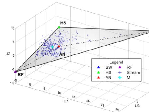
[image:4.612.308.546.368.521.2]

Figure 1.Three-dimensional mixing space generated using stream data, where the median of end-members are projected.U1 repre-sents 59.6 % of the variance,U2 19.7 % andU3 7.4 % (From PCA); RF: rainfall; AN: Andosols; HS: Histosols; SW: spring water;M: the median of stream data (mixture).

Table 1.Median and standard deviation (SD) of end-members and stream projected in three-dimensional space for the study period 2013–2014.

End-member Coordinates∗ Naming in

U1 U2 U3 equations

SW (n=25) median 26.25 7.29 7.00 A

SD 0.46 0.36 0.39

HS (n=33) median 0.23 5.48 1.97 B

SD 0.85 1.29 0.69

AN (n=37) median −2.24 −3.93 3.71 C

SD 0.55 0.58 0.45

RF (n=36) median −5.38 −6.10 −4.84 D

SD 0.27 0.56 0.15

Stream (n=257) median −0.61 −1.04 0.94 M

SD 2.06 1.10 0.66

∗_{Coordinates of end-members and stream (mixture) medians in three-dimensional}

space (U1,U2andU3).nrepresents the sample size.

(5)

[image:5.612.73.521.63.184.2]

Univer-Figure 2.Boxplots of end-members projected in the three-dimensional mixing space for the study period 2013–2014. Theyaxis represents the coordinates of the mixing space and thexaxis the principal componentsU1,U2 andU3 (the central bar in the box represents the median; notches represent the 95 % confidence intervals; whiskers 1.5 times the interquartile range and circles represent outliers). SW: spring water; HS: Histosol; AN: Andosol; RF: rainfall.

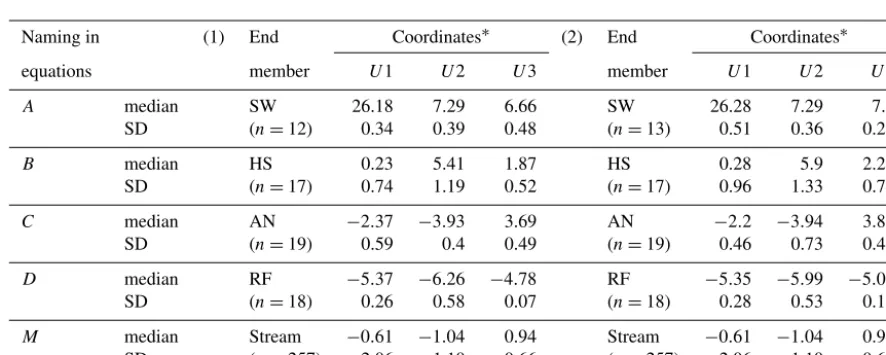
Table 2.Median and standard deviation (SD) of end-members and stream projected in three-dimensional space considering 50 % of the data sets.

Naming in (1) End Coordinates∗ (2) End Coordinates∗

equations member U1 U2 U3 member U1 U2 U3

A median SW 26.18 7.29 6.66 SW 26.28 7.29 7.1

SD (n=12) 0.34 0.39 0.48 (n=13) 0.51 0.36 0.21

B median HS 0.23 5.41 1.87 HS 0.28 5.9 2.26

SD (n=17) 0.74 1.19 0.52 (n=17) 0.96 1.33 0.74

C median AN −2.37 −3.93 3.69 AN −2.2 −3.94 3.89 SD (n=19) 0.59 0.4 0.49 (n=19) 0.46 0.73 0.41

D median RF −5.37 −6.26 −4.78 RF −5.35 −5.99 −5.01 SD (n=18) 0.26 0.58 0.07 (n=18) 0.28 0.53 0.15

M median Stream −0.61 −1.04 0.94 Stream −0.61 −1.04 0.94 SD (n=257) 2.06 1.10 0.66 (n=257) 2.06 1.10 0.66

The example (1) considers the initial 50 % and (2) the remaining 50 % of the sample sets.∗_{Coordinates of end-members and stream (mixture) medians in}

three-dimensional space (U1,U2andU3).nrepresents the sample size.

sity using an ICP-MS (Agilent 7500ce, Agilent Technolo-gies) and the electrical conductivity (EC) was measured in situ. More detailed information on the study site and data set can be found in Correa et al. (2017, 2019b).

3.2 Uncertainty estimation of water source contributions

Using the classic EMMA approach (Christophersen and Hooper, 1992), data from end-members SW, HS, AN, RF and streamMwere projected into a three-dimensional space (Correa et al., 2019b) and presented in Fig. 1. The resulting median and standard deviation of end-members and stream coordinates are shown in Table 1. Furthermore, Fig. 2 shows the distribution of projected samples from individual end-members in the PCA coordinates.

The uncertainty range of each of the four end-member contributions to the stream was determined using the above developed Eq. (15) based on the first-order Taylor series

approximation (Eq. 14) (MATLAB code in Correa et al., 2019a). The fw gives the proportion of w in M and σ_f2_w gives the variances of w. The upper uncertainty limit was computed as fw+t0.05,γσf w and the lower limit as fw− t0.05,γσf w. This procedure was applied to all end-members. The resulting uncertainty estimates for each source end-member are shown in Table 5.

Note that the set of sourcesA,B,CandDused for the de-velopment of the equations are represented here by SW, HS, AN and RF in this specific order.U1,U2 andU3 represent the principal components PC1, PC2 and PC3, respectively.

3.3 Sensitivity of water source uncertainty to input data

[image:5.612.77.520.277.454.2]

(6)

out-Naming in (3) End Coordinates∗ (4) End Coordinates∗

A median SW 26.25 7.3 7.02 SW 26.21 7.29 6.95

SD (n=26) 5.51 1.73 1.68 (n=26) 10.28 2.87 2.54

B median HS 0.27 5.47 1.98 HS 0.23 5.45 1.97

SD (n=34) 0.99 2.45 1.03 (n=34) 1.12 1.99 0.8

The example (3) considers outliers included at the positive extreme of the data set of each source and (4) outliers included at the negative extreme.

[image:6.612.80.518.85.260.2]

∗_{Coordinates of end-members and stream (mixture) medians in three-dimensional space (}_U_1,_U₂_and_U_3)._n_{represents the sample size.}

Table 4.Median and enlarged standard deviation (SD) of end-members and stream projected in three-dimensional space.

Naming in (5) End Coordinates∗ (6) End Coordinates∗

A median SW 26.25 7.29 7.00 SW 26.25 7.29 7.00

SD (n=25) 1.39 1.07 1.19 (n=25) 2.32 1.78 1.99

B median HS 0.23 5.48 1.97 HS 0.23 5.48 1.97

SD (n=33) 2.56 3.87 2.06 (n=33) 4.27 6.45 3.43

The example (5) considers 3 times the standard deviation of the original data set and (6) 5 times the standard deviation of the original data set.∗Coordinates of end-members and stream (mixture) medians in three-dimensional space (U1,U2andU3).nrepresents the sample size.

Table 5.Uncertainty of individual end-member contributions to the stream and Satterthwaite (1946) approximation for the degrees of freedom calculated for the study period 2013–2014.

Naming in equations A B C D

End-member SW HS AN RF

Fraction of end-member contribution 0.06 0.3 0.35 0.29 Upper 95 % confidence limit 0.21 0.57 0.58 0.46 Lower 95 % confidence limit 0.00 0.03 0.12 0.12

Degrees of freedom 291 536 749 628

liers (upper and lower extremes) and the increased standard deviations of the source data sets.

The first example considers 50 % of the samples (collected in the first half of the monitoring period) from each source. The median, standard deviation and sample size are input data (Table 2) to calculate the uncertainty bands (Table 6).

The second example considers the remaining 50 % of the samples and was similarly executed (Table 2).

In the third example, outliers were artificially included at the upper positive end of data sets for each source at each coordinate, respectively. The outliers consisted of twice the maximum positive value of the observed data (Table 3).

Using the same criteria, the negative extremes were in-cluded in the fourth example (Table 3).

[image:6.612.76.519.316.491.2] [image:6.612.46.284.574.654.2]

(7)

[image:7.612.90.507.96.182.2]

Table 6.Uncertainty of individual end-member contributions to the stream and Satterthwaite (1946) approximation for the degrees of freedom computed considering 50 % of the data sets.

Naming in equations (1) A B C D (2) A B C D

End-member SW HS AN RF SW HS AN RF

Fraction of end-member contribution 0.06 0.3 0.35 0.28 0.06 0.28 0.35 0.3 Upper 95 % confidence limit 0.21 0.57 0.58 0.45 0.21 0.55 0.58 0.46 Lower 95 % confidence limit 0.00 0.03 0.12 0.11 0.00 0.02 0.12 0.14

Degrees of freedom 289 493 676 589 288 491 679 537

[image:7.612.91.504.242.327.2]

The example (1) was computed considering the initial 50 % and (2) the remaining 50 % of the sample sets.

Table 7.Uncertainty of individual end-member contributions to the stream and Satterthwaite (1946) approximation for the degrees of freedom computed after including artificial outliers.

The example (3) was computed after including outliers at the positive extreme of the data set and (4) including outliers at the negative extreme.

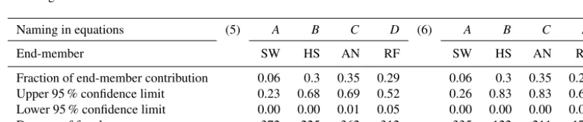
Table 8.Uncertainty of individual end-member contributions to the stream and Satterthwaite (1946) approximation for the degrees of freedom computed with enlarged standard deviations.

The example (5) was computed considering 3 times the standard deviation of the original data set and (6) 5 times the standard deviation of the original data set.

the value of the standard deviation of the initial data set (Ta-ble 4) and finally, increasing the standard deviation 5 times for the sixth example (Table 4).

The results of this analysis are presented in Tables 6–8. In examples 1 and 2 the sample size reduction from 24 to 12 and 13 samples respectively (Table 6) had a minimal effect (less than 3 %) on the calculation of the uncertainty ranges com-pared to the original complete set (Table 1). The fractions of source contributions did not experience changes. The inclu-sion of outliers affected the values of the medians at levels of the second decimal (Table 3) concerning the median of the initial data (Table 2). However, the standard deviations in-creased in a range of 1.2 to 2.5 times the original value for AN and HS, and more for RF (2.5 to 10.5) and drastically more for SW (4 to 20 times wider). These variations were reflected in the widening (1 % to 12 %) of uncertainty bands for all existing cases (Table 7) in comparison with those

cal-culated from the original data set (Table 5). Furthermore, the widening of the standard deviations to 3 and 5 times their ini-tial values resulted in an increase in the range of uncertainty between 2 % and 22 % for the first case and between 5 % and 37 % for the second case. For the latter, the minimum limit of the uncertainty range was reached in all the reported cases. The large number of samples used in these exercises was re-flected in high degrees of freedom.

4 Summary and remarks

[image:7.612.89.505.386.473.2]

(8)

mul-tiple source contributions to a mixture do not experience sig-nificant changes with sample size reduction or inclusion of outliers. Rather, it shows marginally different results by in-corporating standard deviations from widely dispersed data.

The methodology, based on Phillips and Gregg (2001) combined with EMMA applications (Hooper, 2003) presents high potential for use as an alternative method to the simple sum of analytical errors (Uhlenbrook and Hoeg, 2003) or the Bayesian approach (Parnell et al., 2010; Stock et al., 2018). We provide a tool to close the gap in studies of mixing pro-cesses when a larger number of source contributions (>3) and related uncertainty estimates are needed for a more com-plete conceptualization (Iwasaki et al., 2015).

The MATLAB code provided and the illustrative examples facilitate the understanding of the methodology and promote future scientific applications. We are confident that the use of this methodology will help the scientific community that is increasingly using large tracer sets in its research to obtain results supported by a sound uncertainty analysis.

Code and data availability. A MATLAB code to calculate the frac-tions of end-member contribution to the mixture and their associ-ated uncertainties is freely available at https://zenodo.org/record/ 3518700 (last access: 5 November 2019; Correa et al., 2019a), as well as input data (used in this study) as an example for the code run and an instruction note.

Author contributions. AC and CB conceptualized the methodol-ogy. AC was responsible for the data collection and analysis. DOT and AC programmed and evaluated the MATLAB code with col-lected data. AC wrote the paper with contributions from all co-authors.

Competing interests. The authors declare that they have no conflict of interest.

Acknowledgements. Alicia Correa and Christian Birkel would like to acknowledge support by a UCR postdoctoral fellowship awarded to Alicia Correa, UCREA, and the Water and Global Change Ob-servatory at the Department of Geography, UCR. The authors thank the Central Research Office (DIUC) of the Universidad de Cuenca for making available part of the tracer data sets. We are especially grateful for the constructive comments that were provided by the referees, which greatly improved the quality of the technical note.

Review statement. This paper was edited by Markus Hrachowitz and reviewed by two anonymous referees.

Barthold, F. K., Tyralla, C., Schneider, K., Vaché, K. B., Frede, H.-G., and Breuer, L.: How many tracers do we need for end member mixing analysis (EMMA)? A sensitivity analysis, Water Resour. Res., 47, W08519, https://doi.org/10.1029/2011WR010604, 2011.

Barthold, F. K., Turner, B. L., Elsenbeer, H., and Zimmermann, A.: A hydrochemical approach to quantify the role of return flow in a surface flow-dominated catchment, Hydrol. Process., 31, 1018– 1033, https://doi.org/10.1002/hyp.11083, 2017.

Bartov, G., Deonarine, A., Johnson, T. M., Ruhl, L., Vengosh, A., and Hsu-Kim, H.: Environmental Impacts of the Tennessee Val-ley Authority Kingston Coal Ash Spill. 1. Source Apportion-ment Using Mercury Stable Isotopes, Environ. Sci. Technol., 47, 2092–2099, https://doi.org/10.1021/es303111p, 2013.

Belli, R., Borsato, A., Frisia, S., Drysdale, R., Maas, R., and Greig, A.: Investigating the hydrological significance of stalagmite geochemistry (Mg, Sr) using Sr isotope and particulate element records across the Late Glacial-to-Holocene transition, Geochim. Cosmochim. Ac., 199, 247–263, https://doi.org/10.1016/j.gca.2016.10.024, 2017.

Berman, E. S. F., Gupta, M., Gabrielli, C., Garland, T., and McDonnell, J. J.: High-frequency field-deployable isotope analyzer for hydrological applications: RAPID COMMUNICATION, Water Resour. Res., 45, W10201, https://doi.org/10.1029/2009WR008265, 2009.

Bicknell, A. W. J., Knight, M. E., Bilton, D. T., Campbell, M., Reid, J. B., Newton, J., and Votier, S. C.: Intercolony movement of pre-breeding seabirds over oceanic scales: implications of cryp-tic age-classes for conservation and metapopulation dynamics, Divers. Distrib., 20, 160–168, https://doi.org/10.1111/ddi.12137, 2014.

Buytaert, W., Iñiguez, V., Celleri, R., Bièvre, B. D., Wyseure, G., and Deckers, J.: Analysis of the water balance of small páramo catchments in south Ecuador, in: Environmental Role of Wet-lands in Headwaters, Springer, Dordrecht, the NetherWet-lands, 271– 281, 2006.

Christophersen, N. and Hooper, R. P.: Multivariate analysis of stream water chemical data: The use of principal components analysis for the end-member mixing problem, Water Resour. Res., 28, 99–107, https://doi.org/10.1029/91WR02518, 1992. Christophersen, N., Neal, C., Hooper, R. P., Vogt, R. D., and

Ander-sen, S.: Modelling streamwater chemistry as a mixture of soilwa-ter end-members – A step towards second-generation acidifica-tion models, J. Hydrol., 116, 307–320, 1990.

Correa, A., Windhorst, D., Tetzlaff, D., Crespo, P., Célleri, R., Feyen, J., and Breuer, L.: Temporal dynamics in dominant runoff sources and flow paths in the Andean Páramo, Water Resour. Res., 53, 5998–6017, https://doi.org/10.1002/2016WR020187, 2017.

Correa, A., Ochoa-Tocachi, D., and Birkel, C.: MatLab code to cal-culate fractions of contribution to the mixture and associated uncertainties, Zenodo, https://doi.org/10.5281/zenodo.3518700, 2019a.

(9)

headwater catchments, Sci. Total Environ., 651, 1613–1626, https://doi.org/10.1016/j.scitotenv.2018.09.189, 2019b.

Davies, J., Olley, J., Hawker, D., and McBroom, J.: Appli-cation of the Bayesian approach to sediment fingerprint-ing and source attribution, Hydrol. Process., 32, 3978–3995, https://doi.org/10.1002/hyp.13306, 2018.

Delsman, J. R., Essink, G. H. P. O., Beven, K. J., and Stuyfzand, P. J.: Uncertainty estimation of end-member mix-ing usmix-ing generalized likelihood uncertainty estimation (GLUE), applied in a lowland catchment: Uncertainty Estimation of End-Member Mixing, Water Resour. Rese., 49, 4792–4806, https://doi.org/10.1002/wrcr.20341, 2013.

Ehleringer, J. R., Bowen, G. J., Chesson, L. A., West, A. G., Podlesak, D. W., and Cerling, T. E.: Hydro-gen and oxyHydro-gen isotope ratios in human hair are related to geography, P. Natl. Acad. Sci. USA, 105, 2788–2793, https://doi.org/10.1073/pnas.0712228105, 2008.

Falkner, K., Ungerer, C. A., and Christie, D. M.: Inductively Cou-pled Plasma Mass Spectrometry in Geochemistry, Annu. Rev. Earth Pl. Sc., 23, 409–450, 1995.

Genereux, D.: Quantifying uncertainty in tracer-based hy-drograph separations, Water Resour. Res., 34, 915–919, https://doi.org/10.1029/98WR00010, 1998.

Granek, E. F., Compton, J. E., and Phillips, D. L.: Mangrove-Exported Nutrient Incorporation by Sessile Coral Reef Invertebrates, Ecosystems, 12, 462–472, https://doi.org/10.1007/s10021-009-9235-7, 2009.

Helaluddin, A., Khalid, R. S., Alaama, M., and Abbas, S. A.: Main Analytical Techniques Used for Elemental Analy-sis in Various Matrices, Trop. J. Pharm. Res., 15, 427–434, https://doi.org/10.4314/tjpr.v15i2.29, 2016.

Hooper, R. P.: Diagnostic tools for mixing models of stream water chemistry, Water Resour. Res., 39, 1055, https://doi.org/10.1029/2002WR001528, 2003.

Inamdar, S., Dhillon, G., Singh, S., Dutta, S., Levia, D., Scott, D., Mitchell, M., Van Stan, J., and McHale, P.: Temporal variation in end-member chemistry and its influence on runoff mixing pat-terns in a forested, Piedmont catchment, Water Resour. Res., 49, 1828–1844, https://doi.org/10.1002/wrcr.20158, 2013.

Iwasaki, K., Katsuyama, M., and Tani, M.: Contributions of bedrock groundwater to the upscaling of storm-runoff generation pro-cesses in weathered granitic headwater catchments, Hydrol. Pro-cess., 29, 1535–1548, https://doi.org/10.1002/hyp.10279, 2015. James, A. L. and Roulet, N. T.: Investigating the

applicabil-ity of end-member mixing analysis (EMMA) across scale: A study of eight small, nested catchments in a temper-ate forested wtemper-atershed, Wtemper-ater Resour. Res., 42, W08434, https://doi.org/10.1029/2005WR004419, 2006.

Kirchner, J. W. and Neal, C.: Universal fractal scaling in stream chemistry and its implications for solute transport and water quality trend detection, P. Natl. Acad. Sci. USA, 110, 12213– 12218, https://doi.org/10.1073/pnas.1304328110, 2013. Lis, G., Wassenaar, L. I., and Hendry, M. J.: High-Precision

Laser Spectroscopy D/H and18O/16O Measurements of Mi-croliter Natural Water Samples, Anal. Chem., 80, 287–293, https://doi.org/10.1021/ac701716q, 2008.

Liu, F., Williams, M. W., and Caine, N.: Source waters and flow paths in an alpine catchment, Colorado Front

Range, United States, Water Resour. Res., 40, W09401, https://doi.org/10.1029/2004WR003076, 2004.

Magaña-Gallegos, E., González-Zúñiga, R., Cuzon, G., Arevalo, M., Pacheco, E., Valenzuela, M. A. J., Gaxiola, G., Chan-Vivas, E., López-Aguiar, K., and Noreña-Barroso, E.: Nutri-tional Contribution of Biofloc within the Diet of Growout and Broodstock of Litopenaeus vannamei, Determined by Stable Isotopes and Fatty Acids, J. World Aquacult. Soc., 919–932, https://doi.org/10.1111/jwas.12513, 2018.

Mimba, M. E., Ohba, T., Nguemhe Fils, S. C., Wirmvem, M. J., Numanami, N., and Aka, F. T.: Seasonal Hydrological In-puts of Major Ions and Trace Metal Composition in Streams Draining the Mineralized Lom Basin, East Cameroon: Ba-sis for Environmental Studies, Earth Syst. Environ., 1, 1–22, https://doi.org/10.1007/s41748-017-0026-6, 2017.

Padrón, R. S., Wilcox, B. P., Crespo, P., and Célleri, R.: Rainfall in the Andean Páramo: New Insights from High-Resolution Mon-itoring in Southern Ecuador, J. Hydrometeorol., 16, 985–996, https://doi.org/10.1175/JHM-D-14-0135.1, 2015.

Parnell, A. C., Inger, R., Bearhop, S., and Jackson, A. L.: Source Partitioning Using Stable Isotopes: Cop-ing with Too Much Variation, PLOS ONE, 5, e9672, https://doi.org/10.1371/journal.pone.0009672, 2010.

Phillips, D. L. and Gregg, J. W.: Uncertainty in source par-titioning using stable isotopes, Oecologia, 127, 171–179, https://doi.org/10.1007/s004420000578, 2001.

Phillips, D. L. and Gregg, J. W.: Source partitioning using stable isotopes: coping with too many sources, Oecologia, 136, 261– 269, https://doi.org/10.1007/s00442-003-1218-3, 2003. Quichimbo, P., Tenorio, G., Borja, P., Cárdenas, I., Crespo, P., and

Célleri, R.: Efectos sobre las propiedades físicas y químicas de los suelos por el cambio de la cobertura vegetal y uso del suelo: Páramo de Quimsacocha al Sur del Ecuador, Sociedad Colom-biana de la Ciencia del Suelo, 2, 138–153, 2012.

Satterthwaite, F. E.: An Approximate Distribution of Esti-mates of Variance Components, Biometrics Bull., 2, 110–114, https://doi.org/10.2307/3002019, 1946.

Semmens, B. X., Moore, J. W., and Ward, E. J.: Improving Bayesian isotope mixing models: a response to Jackson et al. (2009), Ecol. Lett., 12, E6–E8, https://doi.org/10.1111/j.1461-0248.2009.01283.x, 2009a.

Semmens, B. X., Ward, E. J., Moore, J. W., and Darimont, C. T.: Quantifying Inter- and Intra-Population Niche Variability Us-ing Hierarchical Bayesian Stable Isotope MixUs-ing Models, PLOS ONE, 4, e6187, https://doi.org/10.1371/journal.pone.0006187, 2009b.

Stock, B., Semmens, B., Ward, E., Parnell, A., Jackson, A., and Phillips, D.: MixSIAR: Bayesian Mixing Models in R, available at: https://CRAN.R-project.org/package=MixSIAR (last access: 20 March 2019), 2018.

Taylor, J. R.: An introduction to error analysis. The study of uncertainties in physical measurements, available at: http:// adsabs.harvard.edu/abs/1982aite.book...T (last access: 17 Octo-ber 2018), 1982.

(10)

Walpole, R., Myers, R., Myers, S., and Ye, K.: Proba-bility & Statistics for Engineers & Scientists, MyLab Statistics Update, 9th Edition, Pearson, available at: https://www.pearson.com/us/higher-education/product/Walpole- Probability-and-Statistics-for-Engineers-and-Scientists-9th-Edition/9780321629111.html (last access: 3 September 2019), 2017.