A New Estimator Using Auxiliary Information in Stratified Adaptive Cluster Sampling

(1)

A New Estimator Using Auxiliary Information in Stratified

Adaptive Cluster Sampling

Nipaporn Chutiman*_{, Monchaya Chiangpradit, Sujitta Suraphee} Department of Mathematics, Faculty of Science, Mahasarakham University, Maha Sarakham, Thailand

Email: *[email protected]

Received June 2, 2013; revised July 2, 2013; accepted July 9, 2013

Copyright © 2013 Nipaporn Chutiman et al. This is an open access article distributed under the Creative Commons Attribution Li-cense, which permits unrestricted use, distribution, and reproduction in any medium, provided the original work is properly cited.

ABSTRACT

In this paper, we study the estimators of the population mean in stratified adaptive cluster sampling by using the information of the auxiliary variable. Simulations showed that if the variable of interest (y) and the auxiliary variables (x,z) have high positive correlation then the estimate of the mean square error of the ratio estimators is less than the estimate of the mean square error of the product estimator. The estimators which use only one auxiliary variable were better than the estimators which use two auxiliary variables.

Keywords: Stratified Adaptive Cluster Sampling; Auxiliary Variable; Ratio Estimator; Product Estimator

1. Introduction

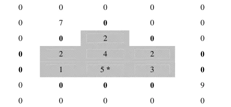
Adaptive cluster sampling, proposed by Thompson [1], is an efficient method for sampling rare and hidden clustered populations. In adaptive cluster sampling, an initial sample of units is selected by simple random sampling. If the value of the variable of interest from a sampled unit satisfies a pre-specified condition , that is , then the unit’s neighborhood will also be added to the sample. If any other units that are “adaptively” added also satisfy the condition , then their neighborhoods are also added to the sample. This process is continued until no more units that satisfy the condition are found. The set of all units selected and all neighboring units that satisfy the condition is called a network. The adaptive sample units, which do not satisfy the condition are called edge units. A network and its associated edge units are called a cluster. If a unit is selected in the initial sample and does not satisfy the condition , then there is only one unit in the network. A neighborhood must be defined such that if unit is in the neighborhood of unit then unit is in the neighborhood of unit . In this paper, a neighborhood of a unit is defined as the four spatially adjacent units, that is to the left, right, top and bottom of that unit as shown in Figure 1.

C



i y, _i c

i



C

i

[image:1.595.308.539.599.706.2]

j j

Figure 1 illustrates the example of a network. The unit with a star is the initial unit selected. The condition to adaptively added units is a value greater than or equal to 1.

Units that are to the left, right, top, and bottom of one another making up a neighborhood. The units in the gray shading form a single network. The units in bold numbers are edge units of the network. The network and its edge units make up a cluster.

Adaptive cluster sampling are applied in stratified random sampling. In adaptive cluster sampling, an initial stratified sample is selected from a population, and whenever the variable of interest for any unit is observed to satisfy the condition, the neighborhood of that unit is added in the sample. Sometimes other variables are re- lated to the variable of interest y. We can obtain additio- nal information for estimating the population mean. The use of an auxiliary variable is a common method to im- prove the precision of estimates of a population mean. In this paper, we will study the estimator of population mean in stratified adaptive cluster sampling using an auxiliary

0 0 0 0 0

0 7 0 0 0

0 0 2 0 0

0 2 4 2 0

0 1 5 * 3 0

0 0 0 0 9

0 0 0 0 0

Figure 1. The example of network where a unit neighbor- hood is defined as four spatially adjacent units.

(2)

variable. Some comparisons are made using a simulation.

2. Stratified Adaptive Cluster Sampling

For stratified adaptive cluster sampling, the population consists of units partitioned into strata based on prior information about units that are similar, and it is assumed that the population ignores crossover between strata. The population in each stratum consists of h units . The population mean of the variable of interest in stratum h is

N



h 1, 2,

L N



L ,   yh

 . An initial sample of unit size h is selected by simple random sampling without replacement and for those units selected that satisfy the condition. Then the unit’s neighborhood is added to the sample.

n Define 1 hi yhi hj j hi w y

m 





is the average of the y-values of the network to which

hi belongs.

u hi is the network that include unit i in stratum

h

and hi is the size of network that include unit in stratum . The estimator of the population mean based on Hansen-Hurwitz estimator (Thompson and Seber [2]) is

m i h _ 1 L h

st a yh

h h N y

n





w (1)

where 1 1 L yh yhi h w w n  



The variance of yst a_ is



_







2

1

1 L yhw

st a h h h

h h

S

V y N N n

N  n





 (2)

where





2

2 1 1 1 h N

yhw yhi yh

h h

S w

N  

  



and 1 h N yh yhi h w N  





_h.

The estimate of V y



st a_



is



_







2

1

ˆ L yhw

st a h h h

h h

s

V y N N n

N  n





 (3)

where





2

2 1 1 1 h n

yhw yhi yh

h h s w n    



3. Propose Estimators

The estimator of the population mean in stratified adaptive cluster sampling using two auxiliary variables (x,z) is (Walid A. Abu-Dayyeh, M. S. Ahmed, R. A. Ahmed and Hassen A. Muttlak, [3]),

1 2

_ _

_ _ _

st a st a st a xz st a

x z x z y y          _ _{ } _  

  (4)

α1 = 0 and α2 = 0 is called mean per unit,α1 = −1 and

2 1 is called multivariate ratio estimator, 1

     1

and 2 1 1

is called multivariate ratio estimator, α1 = 1 and 2 is called multivariate product estimator,

w .

1 1

   and 2 0 is called ratio estimator using x,

and

1 0

  ₂  1 is called ratio estimator using ,

1

z 1

  and 2 0 is called product estimator using x

and ₁ 0 and ₂1 is called product estimator using z.

Let

_ 0

st a y y

y

e 





 , 1 _

st a x

x x e     and _ 2

st a z

z z e     So

 

0

 

1

 

2 0

E e E e E e 

 





2 2

0 0 0

_

_ 2 1 st a y

st a

y y

E e V e E e

y

V  V

     _{ } _        

  y

 

2





2

0 2 2

1

1 L yhw 1

h h h

h h

y y

S

E e N N n A

n

  





  y,





2

1

L

yhw y h h h

h h

S

A N N n

n







Thus

 

2

1 2 x x A E e   ,





2 1 L xhw

x h h h

h h

S

A N N n

n







 

2

2 2 z z A E e   ,





2 1 L zhw

z h h h

h h

S

A N N n

n  



 ,

 





, 0 1 1

1 L xhw yhw 1

h h h x

h

x y h x y

S

E e e N N n A

n

    





  _y









,

0 2

1

1 L yhw zhw 1

h h h y

h

y z h y z

S

E e e N N n A

n

    

(3)

and

 





,

1 2

1

1 L xhw zhw 1

h h h x

h

x z h x z

S

E e e N N n A

n

    





  _z.

So,





 













1 2

_ _ 0 1 2

0 1 1 2 2 1 0 1 2 0 2

1 1 2 2 2 2

1 2 1 2 1 2

1 1 1

1

1 1

2 2

st a xz y

y

y e e e

e e e e e e e

e e e e

                             _{ }  



 



2

_ _ _ _

2 2 2 2 2 2

0 1 1 2 2 1 0 1

2 0 2 1 2 1 2

2 2 2

1 2 1

2 2 2

2 1 2

2

2 2

2

2 2

st a xz st a xz y y

y x z xy

y

x y

y x z

yz xz y z x z

MSE y E y

E e e e e e

e e e e

A A A A

A A                             _       _{ }   _        _  

To find 1 and 2 which minimizes MSE y



st a xz_ _



take partial derivative of MSE y



st a xz_ _



with respect to

1

 , 2and set it equal to zero.



_ _



1

0 st a xz

MSE y     and



_ _



2 0 st a xz

MSE y

 

 

So the optimum values of 1 and 2 are

1 2

x xy x xz x y x z

A A A A          _  _   and









2 ₂

xy xz x yz z

y x z xz

A A A A A A A

     

The estimate of 1 is

1 2

ˆ ˆ

x xy x xz

x y x z

A A A A                 

and the estimate of 2 is









2 ₂

ˆ ˆ ˆ ˆ

ˆ

ˆ ˆ ˆ

xy xz x yz z

y x z xz

A A A A A A A

      where





2

1

ˆ L xhw

x h h h

h h

s

A N N n

n





 ,





2

1

ˆ L zhw

z h h h

h h

s

A N N n

n





 ,





,

1

ˆ L xhw yhw

xy h h h

h h

s

A N N n

n





 ,





,

1

ˆ L xhw zhw

xz h h h

h h

s

A N N n

n  



 and





, 1

ˆ L yhw zhw

xy h h h

h h

s

A N N n

n





 .

4. Simulation Study

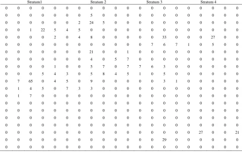
This section, the simulation x-values z-values and y-values fromChutiman, N. and Kumphon, B. [4]were stu- died. The data partition into 4 stratum. The stratum size is 20 × 5 = 100 units. The populations were shown in

Figures 2-4. Sample of units is selected by simple ran-dom sampling without replacement. The y-values are obtained for keeping the sample network. In each the sample network, the x-values and z-values are obtained. The condition for added units in the sample is defined by



: 0



C y y .

For each estimator 5000 iterations were performed to obtain an accuracy estimate. Initial SRS sizes were varied h = 5, 10, 15, 20 and 30 were used. The esti- mated mean square error of the estimate mean is

n

 

5000





₂

1

1 ˆ

5000 i i y

MSE y y 





 ,

where yi is the value for the relevant estimator for sample i.

The estimate of the mean square of the estimators



 1 2



are shown in Table 1, where

ˆ

MSE y 10 and

2 0

  is called MSEˆ of mean per unit, 1 1 and

2 1

   is called MSEˆ of multivariate ratio estimator,

1 1

   and 2  1 is called MSEˆ of multivariate

ratio estimator, ₁1 and 21 is called MSEˆ of multivariate product estimator, 1 1 and 20 is called MSEˆ of ratio estimator using x, 10 and

2 1

   is called MSEˆ of ratio estimator using , 1

z 1

  and 20 is calledMSEˆ of product estimator

using x and 10 and 21 is called MSEˆ of product estimator using z.

5. Conclusion

(4)

Stratum1 Stratum 2 Stratum 3 Stratum 4

0 0 0 0 0 0 0 0 0 0 0 0 0 0 0 0 0 0 0 0

0 0 0 0 0 0 0 5 0 0 0 0 0 0 0 0 0 0 0 0

0 0 0 0 0 0 2 24 5 0 0 0 0 0 0 0 0 0 0 0

0 0 1 22 5 4 5 0 0 0 0 0 0 0 0 0 0 0 0 0

0 0 0 0 2 0 4 8 0 0 0 0 0 33 0 0 0 27 0 0

0 0 0 0 0 0 0 0 0 0 0 0 7 6 7 1 0 5 0 0

0 0 0 0 0 0 0 21 0 0 1 0 0 0 0 0 0 0 0 0

0 0 0 0 0 0 0 4 0 5 7 0 0 0 0 0 0 0 0 0

0 0 0 0 1 0 0 5 7 0 7 7 6 3 0 0 0 0 0 0

0 0 0 5 4 3 0 5 8 4 5 1 0 5 0 0 0 0 0 0

0 7 65 0 4 5 0 9 0 0 0 0 0 3 1 0 0 0 0 0

0 1 4 5 0 7 3 3 0 0 0 0 0 0 0 0 0 0 0 0

0 1 7 0 0 0 0 0 0 0 0 0 0 0 0 0 0 0 0 0

0 0 0 0 0 0 0 0 0 0 0 0 0 0 0 0 0 0 0 0

0 0 0 0 0 0 0 0 0 0 0 0 0 0 0 0 27 0 0 21

0 0 0 0 0 0 0 0 0 0 0 0 0 29 0 0 0 0 0 0

[image:4.595.56.536.87.390.2]

0 0 0 0 0 0 0 0 0 0 0 0 0 0 0 0 0 0 0 0

Figure 2. Y values.

0 0 0 0 0 0 0 0 0 0 0 0 0 0 0 0 0 0 0 0

0 0 0 0 0 0 0 2 0 0 0 0 0 0 0 0 0 0 0 0

0 0 0 0 0 0 1 11 3 0 0 0 0 0 0 0 0 0 0 0

0 0 0 11 2 2 1 0 0 0 0 0 0 0 0 0 0 0 0 0

0 0 0 0 1 0 2 4 0 0 0 0 0 12 0 0 0 15 0 0

0 0 0 0 0 0 0 0 0 0 0 0 3 2 3 0 0 2 0 0

0 0 0 0 0 0 0 16 0 0 0 0 0 0 0 0 0 0 0 0

0 0 0 0 0 0 0 2 0 2 3 0 0 0 0 0 0 0 0 0

0 0 0 0 0 0 0 2 2 0 3 3 2 1 0 0 0 0 0 0

0 0 0 2 2 1 0 2 3 2 2 0 0 2 0 0 0 0 0 0

0 3 18 0 2 2 0 4 0 0 0 0 0 1 0 0 0 0 0 0

0 0 2 2 0 3 1 1 0 0 0 0 0 0 0 0 0 0 0 0

0 0 3 0 0 0 0 0 0 0 0 0 0 0 0 0 0 0 0 0

0 0 0 0 0 0 0 0 0 0 0 0 0 0 0 0 0 0 0 0

0 0 0 0 0 0 0 0 0 0 0 0 0 0 0 0 12 0 0 12

0 0 0 0 0 0 0 0 0 0 0 0 0 27 0 0 0 0 0 0

0 0 0 0 0 0 0 0 0 0 0 0 0 0 0 0 0 0 0 0

[image:4.595.58.537.94.715.2]

(5)

0 0 0 0 0 0 0 0 0 0 0 0 0 0 0 0 0 0 0 0 0 0 0 0 0 0 0 9 0 0 0 0 0 0 0 0 0 0 0 0

0 0 0 1 0 0 12 77 8 0 0 0 0 0 0 0 0 0 0 0

0 0 0 57 10 8 14 0 0 0 0 0 0 0 0 0 0 0 0 0

0 0 0 0 10 0 10 8 0 0 0 0 0 55 1 0 0 97 0 0 0 0 0 0 0 0 0 0 0 0 0 0 17 6 6 1 0 9 0 0 0 0 0 0 0 0 0 74 0 0 0 0 0 0 0 0 0 0 0 0

0 0 0 0 0 0 0 11 0 10 11 0 0 0 0 0 0 0 0 0

0 0 0 0 1 0 0 12 12 0 10 10 12 12 0 0 0 0 0 0

0 0 0 6 8 12 0 12 8 12 10 0 0 10 0 0 0 0 0 0

0 8 53 0 8 6 0 8 0 0 0 0 0 10 0 0 0 0 0 0

0 0 14 10 0 8 12 14 0 0 0 0 0 0 0 0 0 0 0 0

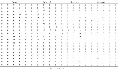
[image:5.595.61.537.81.360.2]

0 0 12 0 0 0 0 0 0 0 0 0 0 0 0 0 0 0 0 0 0 0 0 0 0 0 0 0 0 0 0 0 0 0 0 0 0 0 0 0 0 0 0 0 0 0 0 0 0 0 0 0 0 0 0 0 0 0 0 0 0 0 0 0 0 0 0 0 0 0 0 0 0 0 0 0 0 0 0 0 0 0 0 0 0 0 0 0 0 0 0 0 0 0 0 0 0 0 0 0 0 0 0 0 0 0 0 0 0 0 0 0 0 0 0 0 59 0 0 54 0 0 0 0 0 0 0 0 0 0 0 0 0 63 0 0 0 0 0 0 0 0 0 0 0 0 0 0 0 0 0 0 0 0 0 0 0 0 0 0

Figure 4. Z values.

Table 1. The estimate mean square error of the estimators.

h

n n MSE yˆ

 

 00 MSE yˆ

 

 10 MSE yˆ

 

10 MSE yˆ

 

 01

 

 0 1 ˆ

MSE y MSE yˆ

 

 11 MSE yˆ

 

 1 1

 

 * * 12

ˆ MSE y

 

5 20 0.8105 8.2450 0.1341 7.3278 0.1589 79.6045 5.7501 1.9343

10 40 0.3212 2.1277 0.0397 1.8104 0.0427 10.0623 2.7507 0.9560

15 60 0.1935 1.3305 0.0239 0.9954 0.0189 4.7206 0.6095 0.6242

20 80 0.1104 0.5740 0.0204 0.4883 0.0146 1.6832 0.4179 0.3891

25 100 0.0744 0.4013 0.0190 0.3362 0.0130 1.0909 0.2390 0.2796

30 120 0.0619 0.3207 0.1154 0.2825 0.0081 0.8702 0.1537 0.2221

40 160 0.0442 0.2242 0.0105 0.1927 0.0049 0.5527 0.1194 0.1595

terest

 

y and the auxiliary variables



x z,



have high positive correlation then the estimate of the mean square error of the ratio estimators is less than the estimate of the mean square error of the product estimator. The estimators which use only one auxiliary variable were better than the estimators which use two auxiliary variables.

6. Acknowledgements

This research was supported by Faculty of science Maha- sarakham University, Thailand. We would also like to profoundly thank Mr. Paveen Chutiman for his program- ming advice.

REFERENCES

[1] S. K. Thompson, “Adaptive Cluster Sampling,” Journal

of the American Statistical Association, Vol. 85, No. 412, 1990, pp. 1050-1059.

doi:10.1080/01621459.1990.10474975

[2] S. K. Thompson and G. A. F. Seber, “Adaptive Sam-pling,” Wiley, New York, 1996.

[3] W. A. Abu-Dayyeh, M. S. Ahmed, R. A. Ahmed and H. A. Muttlak, “Some Estimators of a Finite Population Mean Using Auxiliary Information,” Applied Mathemat-

ics and Computation, Vol. 139, No. 2-3, 2003, pp. 287- 298. doi:10.1016/S0096-3003(02)00180-7

[4] N. Chutiman and B. Kumphon, “Ratio Estimator Using Two Auxiliary Variables for Adaptive Cluster Sampling,”

[image:5.595.59.539.394.507.2]