Weibull Bayesian Estimation Based on Maximum Ranked Set Sampling with Unequal Samples

http://www.scirp.org/journal/ojs ISSN Online: 2161-7198

ISSN Print: 2161-718X

Weibull-Bayesian Estimation Based on Maximum

Ranked Set Sampling with Unequal Samples

B. S. Biradar

1

, B. K. Shivanna

2*

1_{Department of Studies in Statistics, University of Mysore, Mysuru, India} 2_{Department of Statistics, Maharani’s Science College for Women, Mysuru, India}

Abstract

A modification of ranked set sampling (RSS) called maximum ranked set sampling with unequal sample (MRSSU) is considered for the Bayesian estimation of scale pa-rameter α of the Weibull distribution. Under this method, we use Linex loss func-tion, conjugate and Jeffreys prior distributions to derive the Bayesian estimate of α. In order to measure the efficiency of the obtained Bayesian estimates with respect to the Bayesian estimates of simple random sampling (SRS), we compute the bias, mean squared error (MSE) and asymptotic relative efficiency of the obtained Bayesian es-timates using simulation. It is shown that the proposed eses-timates are found to be more efficient than the corresponding one based on SRS.

Keywords

Bayesian Estimation, Loss Function, MRSSU, SRS, RSS

1. Introduction

In certain practical problems, actual measurements of a variable interest are costly or time-consuming, but the ranking items according to the variable is relatively easy with- out actual measurement. Under such circumstances McIntyre [1] proposed a sampling scheme called ranked-set sampling (RSS) which can be employed to gain more information than simple random sampling (SRS), while keeping the cost of, or the time constraint on, the sampling about the same. In RSS; one first draws 2

m units at

random from the population and partition them into m sets of m units. The m units in each set are ranked without making, an actual measurement. The first set of m units are ranked and the smallest is selected for actual quantification. From the second set of m

units, the unit ranked and the second smallest is measured, and so on. This method of selection continues until the unit ranked largest is measured from the m-th set. If a

How to cite this paper: Biradar, B.S. and Shivanna, B.K. (2016) Weibull-Bayesian Es- timation Based on Maximum Ranked Set Sampling with Unequal Samples. Open Journal of Statistics, 6, 1028-1036.

http://dx.doi.org/10.4236/ojs.2016.66083 Received: September 20, 2016

Accepted: November 26, 2016 Published: December 2, 2016 Copyright © 2016 by authors and Scientific Research Publishing Inc. This work is licensed under the Creative Commons Attribution International License (CC BY 4.0).

http://creativecommons.org/licenses/by/4.0/

large sample is required, then the procedure can be repeated r times to obtain a sample of size n=rm. These chosen elements are called ranked set sampling. The mathe-

matical support and statistical theory was provided by Takahasi and Wakimoto [2]. Dell and Clutter [3] studied theoretical aspects of this technique on the assumption of perfect and imperfect judgment ranking. Shaibu and Muttlak [4] used median and extreme ranked set sampling method for estimating the parameters of normal, expo- nential and gamma distributions. Al-Omari et al. [5] Used extreme ranked set sampling method to find the estimates of the population mean. Islam et al. [6] Obtained the modified maximum likelihood estimator of location and scale parameters depend on selected ranked set sampling for normal distribution. Ibrahim and Syam [7] used stratified median ranked set sampling method for estimating the population mean.

Some research works have investigated ranked set sampling from a Bayesian point of view. Varian [8] and Zellner [9] introduced Bayesian estimation by using asymmetric loss functions. Al-Saleh and Muttlak [10] obtained the Bayesian estimates of the exponential distribution. Ahmed [11] obtained the Bayesian estimators of log-normal distribution based on RSS and SRS using Bayes risk. Sadek et al. [12], and Sadek and Alharbi [13] used the asymmetric loss function to obtain the Bayesian estimate of the exponential and Weibulldistributions respectively, based on SRS and RSS. Al-Hadhrami and Al-Omari [14] showed that the Bayesian estimation of the mean of normal distri- bution based on moving extreme ranked set sampling (MERSS) is more efficient than SRS. Hassan [15] obtained the maximum likelihood estimator and Bayesian estimates of shape and scale parameters of the exponentiated exponential distribution based on SRS and RSS. For more research work on Bayesian one may refer to Mohammadi and Pazira [16], Ghafoori et al. [17], Said Ali Al-Hadhrami and Amer Ibrahim Al-Omari

[18], Mohie El-Din et al. [19].

In this paper, we derive the Bayesian estimates of the Weibull scale parameter α

based on gamma and Jeffreys prior distributions by MRSSU method proposed by Biradar and Santosha [20]. In Section 2, the preliminaries are discussed. The Bayesian estimates under SEL and LINEX loss functions of the parameter of Weibull distribution using SRS and MRSSU are presented in Section 3. Simulation results and Conclusions are presented in Section 4 and 5 respectively.

2. Preliminaries

Let X X1, 2,,Xm be a sequence of independent and identically distributed (iid)

random variables from a Weibull distribution with probability density function (pdf)

( )

1

= e x , 0, > 0, > 0

f x αβxβ− −α β x≥ α β (1)

And cumulative distribution function (cdf)

(

, ,

)

1 e x , 0, > 0.

F xα β = − −αβ x≥ α (2)

where

α

is the scale parameter and β is shape parameter.

The Linex loss function for the parameter

α

_{can be expressed as}

( )

(

ec 1 ,

)

L ∆ =d ∆ − ∆ −c

where ∆ =

(

α αˆ−

)

;

α

ˆ is an estimate of

α

and, c and d are shaped and scale parameters. The sign and magnitude of the shape parameter c indicate that the direction and degree of symmetry, respectively. When the value of c is zero, the Linex loss function is approximately squared error loss, when c is less than zero, the Linex loss function gives more weight to under-estimation against over-estimation, and it is reversed whenc value is greater than zero. The conjugate prior for

α

_, Gamma a b

( )

,

is considered, whose pdf is given by

( )

_{( )}

1e , 0 ,

a b

bαα α

π α α

α

− −

= < < ∞

Γ (3)

where a b, >0. If a= =b 0, then π α

( )

becomes the Jeffreys prior.

3. Bayesian Estimates

In this section, we derive the Bayes estimates of the Weibull parameter

α

based on simple random sampling and maximum ranked set sampling with unequal samples by assuming that the shape parameter β is known. In each case, we use both conjugate and non-informative prior for the scale parameter

α

. Also, we use the symmetric loss function (squared error loss) and asymmetric loss function (Linear-exponential, Linex) to derive the corresponding Bayesian estimates. And we denote k

(

α|X

)

and k

(

α|Y

)

as posterior densities of

α

, given SRS(X) and RSS(Y) respectively.

3.1. Bayesian Estimation Based on SRS

Let X X1, 2,,Xm be a sequence of iid random variables, has the Weibull distribution

with parameters (α β, ) and π α

( )

be the conjugate prior. In this case, the posterior

density based on SRS is given by

(

)

( )

(

)

1 1

1 e

| .

m i i

m a

b x m

m a

i i

b x

k x

m a

β

α

β

α α

=

  ₊

− _ + _

+ −  

=

∑ _{ }

+

 

 

=

Γ +

∑

(4)

Hence, the Bayesian estimation of

α

depend on squared error loss (SEL) is

(

)

*

|

Sel E X

θ

=

θ

because the Bayes estimate with respect to SEL is the posterior mean then

( )

(

)

*

0

1

| d .

Sel m

i i m a

X k x

b xβ

α ∞α α α

=

+

= =

+

∫

∑

(5)

While the Bayesian estimate of

α

based on Linex loss function is

( )

* 1

ln ec

Lnx E

c

α

α

_{= − } − _

 

( )

₍

₎

1 1 0 1 e d e n i i

m a _{b x}

n m a i i c b x E m a β α β α α α =   + _{−  + }   ∞ _{  + −} = − ∑  ₊      = Γ +

∑

∫

Then,

( )

( ) * 1 1 1 ln . m a n i i lnx n i i b x X c

b x c

β β α + = =  ₊      = −  _{+ +}     

∑

∑

(6)

3.2. Bayesian Estimation Based on MRSSU

Assume that the variable of interest X has density function f x

(

|α

)

and distribution

function F x

(

|α

)

is known. Let

{

X_i1,X_i2,,X_ii

}

, i=1,,m be m sets of random

samples from X, and they are independent. Denote, Yi=Max

{

Xi1,Xi2,,Xii

}

,

1, ,

i=  m. Let Y₁ is taken from the first set, Y2 is taken from the second set and Ym

is taken from the last set, then

{

Y Y1, 2,,Ym

}

be a one cycle MRSSU from X and all i

Y’s are independent. In this study we assume that there is no error in ranking. The

density of Yi has the same density as the ith order statistic (maximum) of an SRS of

size i from f y

(

,α

)

, i.e., Y_i has the density

(

)

(

)

1

(

)

| , i , .

i

f y α = i F y_ α _− f yα

Let MRSSU be drawn from Weibull distribution, then the density function of Yi is

(

)

1 1

( )

( )

1

1 1

0

1

| 1 e i e i 1 e i .

i i

q

y y y q

i i i

q i

f y i y i y

q

β β β

α β α β α

α − − αβ − − − αβ − − +

= −     = _ − _ = _{ } −  

∑

Then the joint density of MRSSU in this case due to independence of yi’s is given by

(

)

(

)

( )

( )

( )

( )

1 2 1 1 1 0 1 1

0 1 1

1

0 0 0 1 1

1

| | 1 e

, 0

i

m

m m i

q y q

i i q i i m m m m m

k k i i

k k k i i

i

g y f y i y

q

A i D i y y

β

α β

β

α θ αβ

α β − − + − = = = − − = = = = = −   = = _{ } −    

= _{ } >

 

∑

∏

∏

∑ ∑ ∑ ∏



∏

where

( )

1

( )

1ki

k

i i A i i

k

−

 

= _{ } −

  and

( )

( )

1 1

e mi yi ki k

D i = −α∑= β + _.

Then the posterior density of α is

( )

( )

( )

( )

( )

( )

( )

( )

( )

( )

1 1 2 1 1 2 1 2 1

0 1 1

1 0 0 0 1

1

0 1 1

1 0

0 0 0 0 1

0 1 1

0 0 0 1

e | | | d e d m i i i m m i i i m m

y k b m

m

m a k

k k k i

y k b m

m

m a k

k k k i

m m

m a k

k k k i

A i g y k y g y A i A i β β α α α

π α α

α

π α α α

α α α = =   − + + − _ _ + −   = = = = ∞   − + + − _∞ _ _ + −   = = = = − + = = = = ∑ ∑       = =             =

∑ ∑ ∑ ∏

∫

_{∑ ∑ ∑ ∏}

_∫

∑ ∑ ∑ ∏

   ( )

( ) (

)

(

)

( ) 1 1 1

0 1 1

e . 1 m i i i

y k b

m a m

m m

A i m a y k b

β α β =   − _ + + _ −   − + − ∑

 _{Γ +}  _{+ +} 

 

 

∑ ∑ ∑



∏

∑

The Bayes estimate of

α

_{based on the squared error loss function is}

( )

(

)

( )

( )

( )

( ) (

)

(

)

( )

( ) (

)

1 1 2 1 2 1 2 0 1

0 1 1

1 0

0 0 0 1

0 1 1

0 0 0 1 1

0 1 1

0 0 0 1

| | d

e d 1 m i i i m m m Sel

y k b c m

m

m a k

k k k i

m a m

m m

k i i

k k k i i

m m

k

k k k i i

Y E Y k y

A i

A i m a y k b

A i m a

β

α

β

α α α α α

α = α

∞   − + + + − _∞ _ _ + −   = = = = − + − = = = = = − = = = = = ∑ = =       =

 _{Γ +}  _{+ +} 

    _{ }     ₊     =

∫

∑ ∑ ∑ ∏

∫

∑ ∑ ∑

∏

∑

∑ ∑ ∑ ∏

   

(

)

( )

( )

(

)

( ) 1 2 1 1

0 1 1

0 0 0 1 1

1 . 1 m m a m i i m a m m m

k i i

k k k i i

y k b

A i y k b

β β − + + − + − = = = = =  _{+ +}         _{+ +}     _{  }  

∑

∑ ∑ ∑



∏

∑

(8)

Next, in order to derive the Bayesian estimation of

α

based on LINEX loss function, first we need to compute the posterior expectation of e−cα _{from Equation (7) as}

( )

( )

(

)

( )

( )

(

)

( )

1 2

1 2

0 1 1

0 0 0 1 1

0 1 1

0 0 0 1 1

1 e . 1 m m m a m m m

k i i

k k k i i

c

m a m

m m

k i i

k k k i i

A i y k b c

E

A i y k b

β α β − + − = = = = = − − + − = = = = =    _{+ + +}     _{  }   =    _{+ +}     _{  }  

∑ ∑ ∑

∏

∑

∑ ∑ ∑

∏

∑

  (9)

Now the Bayesian estimation of

α

on LINEX is

( )

1

ln e c .

Lnx E

c

α

α

_{= − } − _

 

 (10)

where E_e−cα_ is as derived in Equation (9).

3.3. Bayesian Estimation Based on Non-Informative Prior

The non-informative prior distribution of the parameter

α

is obtained from Equation (3) and it is given by

π α

( )

1,

α

0

α

∝ > . Then, we obtain the Bayesian estimates of

α

in this case as follows:

1) Simple Random Sample:

( )

* 1 . j Sel m i i m X x α = =

∑

(11)

and

( )

* 1 1 1 ln . m n i j i Lnx n i i x X c x c β β α = =       = −  ₊     

∑

∑

(12)

2) Maximum ranked set sampling with unequal samples:

( )

( )

(

)

( )

( )

(

)

1 2 1 2 1

0 1 1

0 0 0 1 1

0 1 1

0 0 0 1 1

1 . 1 m m m m m m

k i i

k k k i i

j

Sel _{m m m} m

k i i

k k k i i

A i m y k Y

A i y k

and

.

1))

(

(

)

(

)

1)

(

(

)

(

1

=

~

1 = 1

= 1

0 = 1

0 = 2 0

0 = 1

1 = 1

= 1

0 = 1

0 = 2 0

0 = 1





























+













+

+













−

− −

− −

∑

∏

∑

∑

∑

∑

∏

∑

∑

∑

m i

i m

i k m

i m

m k k k

m i

i m

i k m

i m

m k k k j

Lnx

k

y

i

A

c

k

y

i

A

ln

c

_β

β

α





(14)

4. Simulation Results

To illustrate the performance of the derived Bayesian estimates of scale parameter

( )

α of the Weibull distribution with informative and non-informative prior based on SRS and MRSSU, we carry out the Monte Carlo simulations using R-Software version 3.1.1. We compute bias, mean squared error and relative efficiency of the estimators by assuming the shape parameter β

(

=0.5

)

is known. The numerical results obtained for

[image:6.595.212.559.86.167.2] [image:6.595.195.555.377.519.2]

fixed values of

α

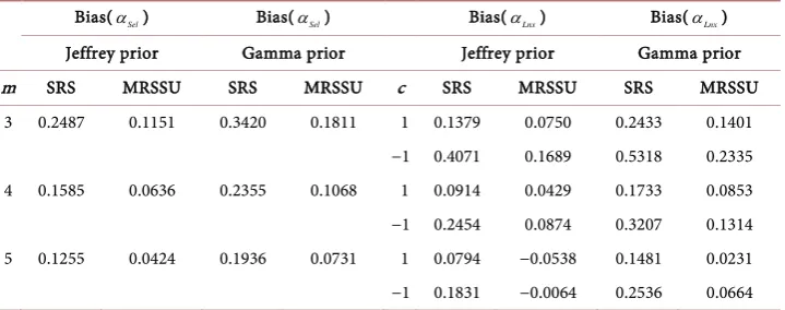
_{, [}α =0.5 and 1] and sample size m [3, 4 and 5] for 1000 runs. The bias of the Bayesian estimates based on SRS and MRSSU are presented in Table 1 and

Table 2, and MSE of the Bayesian estimates based on SRS and MRSSU is presented in

Table 3 and Table 4.

Table 1. Bias of the Bayesian estimates based on SRS and MRSSU. For α=0.5 (when β=0.5, 1

a= , b=0.5).

Bias(αSel) Bias(αSel) Bias(αLnx) Bias(αLnx)

Jeffrey prior Gamma prior Jeffrey prior Gamma prior m SRS MRSSU SRS MRSSU c SRS MRSSU SRS MRSSU

[image:6.595.194.555.564.707.2]

3 0.2487 0.1151 0.3420 0.1811 1 0.1379 0.0750 0.2433 0.1401 −1 0.4071 0.1689 0.5318 0.2335 4 0.1585 0.0636 0.2355 0.1068 1 0.0914 0.0429 0.1733 0.0853 −1 0.2454 0.0874 0.3207 0.1314 5 0.1255 0.0424 0.1936 0.0731 1 0.0794 −0.0538 0.1481 0.0231 −1 0.1831 −0.0064 0.2536 0.0664

Table 2. Bias of the Bayesian estimates based on SRS and MRSSU. For α=1 (when β=0.5, 1

a= , b=0.5).

Bias(αSel) Bias(αSel) Bias(αLnx) Bias(αLnx)

Jeffrey prior Gamma prior Jeffrey prior Gamma prior m SRS MRSSU SRS MRSSU c SRS MRSSU SRS MRSSU

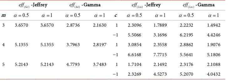
The relative efficiency of the Bayesian estimates based on maximum ranked set sampling with unequal samples with respect to simple random sampling can be defined as follows

( )Sel SRS

(

₍

Sel

)

₎

and (Lnx) SRS

(

₍

Lnx

)

₎

MRSSU Sel MRSSU Lnx

MSE MSE

eff eff

MSE MSE

α α

α α

= =

[image:7.595.194.555.216.359.2]

And are presented in Table 5.

Table 3. MSE of the Bayesian estimates based on SRS and MRSSU. For α=0.5 (when β=0.5, 1

a= , b=0.5).

MSE(αSel) MSE(αSel) MSE(αLnx) MSE(αLnx)

Jeffrey prior Gamma prior Jeffrey prior Gamma prior m SRS MRSSU SRS MRSSU c SRS MRSSU SRS MRSSU

[image:7.595.193.555.404.547.2]

3 0.4193 0.1147 0.3899 0.1357 1 0.1849 0.0800 0.2179 0.0980 −1 1.0296 0.1870 1.2535 0.2015 4 0.2850 0.0555 0.2470 0.0651 1 0.1389 0.0450 0.1524 0.0528 −1 0.4709 0.0712 0.4577 0.0823 5 0.1584 0.0304 0.1696 0.0355 1 0.1004 0.0387 0.1170 0.0505 −1 0.2593 0.0615 0.2823 0.0542

Table 4. MSE of the Bayesian estimates based on SRS and MRSSU. For α=1 (when β=0.5, 1

a= , b=0.5).

MSE(αSel) MSE(αSel) MSE(αLnx) MSE(αLnx)

Jeffrey prior Gamma prior Jeffrey prior Gamma prior m SRS MRSSU SRS MRSSU c SRS MRSSU SRS MRSSU

3 1.6772 0.4586 0.8381 0.3874 1 0.4288 0.2397 0.3299 0.2208 −1 3.9104 1.2337 3.8436 0.8687 4 1.1400 0.2220 0.5929 0.2103 1 0.3550 0.1507 0.2771 0.1453 −1 3.0419 0.3914 1.7406 0.3360 5 0.6337 0.1215 0.4605 0.1228 1 0.2852 0.1327 0.2464 0.1168 −1 1.6544 0.3654 1.0991 0.2718

Table 5. Relative efficiency when α=0.5 and α=1.

( )Sel

eff -Jeffrey eff_{( )}Sel -Gamma eff(Lnx)-Jeffrey eff(Lnx)-Gamma m α=0.5 α=1 α=0.5 α=1 c α=0.5 α=1 α=0.5 α=1

[image:7.595.193.557.578.707.2]

5. Conclusions

We present Bayesian estimation based on SRS and MRSSU. The Weibull distribution is used as an application example to illustrate our results. We compute bias, MSE and relative efficiency of the derived Bayesian estimates and then make a comparison between SRS and MRSSU. Our observations of the results are stated in the following points:

1) From Table 1 and Table 2, first, we found that the Bayesian estimates of

α

are all biased. Next, we found that the Bayesian estimates based on Jeffreys prior are less biased than gamma prior. Also, we observed that the Bayesian estimates based on MRSSU are considerably less biased than SRS.

2) From Table 3 and Table 4, it is observed that the mean squared error of all estimates decreases when sample size m increases. Next, we observed that the Bayesian estimates based on MRSSU have a much smaller mean squared error than the corresponding Bayesian estimates based on SRS in all cases considered.

3) From Table 5, we observe that the relative efficiency of the Bayesian estimator based on MRSSU w.r.t. SRS Bayesian estimators are greater than 1 and increases with

m. Also, decreases in Linex function as m increases for m=5.

Therefore, we conclude that the Bayesian estimates based on maximum ranked set sampling with unequal samples are more efficient than the corresponding Bayesian estimates of simple random sampling.

Finally, we conclude that the results of the simulation experiment showed that the Bayesian estimates based on maximum ranked set sampling with unequal samples are more efficient, when compared with the Bayesian estimates of simple random sam-pling.

Acknowledgements

The authors would like to thank the referees for their helpful comments that have led to an improved paper.

References

[1] McIntyre, G.A. (1952) A Method for Unbiased Selective Sampling Using Ranked Sets. Aus-tralian Journal of Agricultural Research, 3, 385-390. https://doi.org/10.1071/AR9520385

[2] Takahasi, K. and Wakimoto, K. (1968) On Unbiased Estimates of the Population Mean Based on the Sample Stratified by Means of Ordering. Annals of the Institute of Statistical Mathematics, 20, 1-31. https://doi.org/10.1007/BF02911622

[3] Dell, T.R. and Clutter, J.L. (1972) Ranked Set Sampling Theory with Order Statistics Back-ground. Biometrics, 28, 545-555. https://doi.org/10.2307/2556166

[4] Shaibu, A.B. and Muttlak, H.A. (2004) Estimating the Parameters of the Normal, Exponen-tial and Gamma Distributions Using Median and Extreme Ranked Set Samples. Statistics, 1, 75-98.

[6] Islam, T., Shaibur, M.R. and Hossain, S.S. (2009) Effectivity of Modified Maximum Like-lihood Estimators Using Selected Ranked Set Sampling Data. Austrian Journal of Statistics, 38, 109-120.

[7] Ibrahim, K. and Syam, M. (2010) Estimating the Population Mean Using Stratified Median Ranked Set Sampling. Applied Mathematical Sciences, 4, 2341-2354.

[8] Varian, H.R. (1975) A Bayesian Approach to Real Estate Assessment. North Holland, Ams-terdam, 195-208.

[9] Zellner, A. (1986) Bayesian Estimation and Prediction Using Asymmetric Loss Functions. Journal of the American Statistical Association, 81, 446-451.

https://doi.org/10.1080/01621459.1986.10478289

[10] Al-Saleh, M.F. and Muttlak, H.A. (1998) A Note in Bayesian Estimation Using Ranked Set Sampling. Pakistan Journal of Statistics, 14, 49-56.

[11] Ahmed (2007) Bayesian Estimation of the Logormal Distrbution Mean Using Ranked SET Sampling. Basrah Journal of Science, 25, 101-112.

[12] Sadek, A., Sultan, K.S. and Balakrishnan, N. (2009) Bayesian Estimation Based on Ranked Set Sampling Using Asymmetric Loss Function. Bulletin of the Malaysian Mathematical Sciences Society, 38, 707-718.

[13] Sadek, A. and Alharbi, F. (2014) Weibull-Bayesian Analysis Based on Ranked Set Sampling. International Journal of Advanced Statistics and Probability, 2, 114-123.

http://dx.doi.org/10.14419/ijasp.v2i2.3373

[14] Al-Hadhrami, S.A. and Al-Omari, A.I. (2009) Bayesian Inference on the Variance of Nor-mal Distribution Using Moving Extremes Ranked Set Sampling. Journal of Modern Ap-plied Statistical Methods, 8, 273-281.

[15] Hassan, A.S. (2013) Maximum Likelihood and Bayes Estimators of the Unknown Parame-ters for Exponentiated Exponential Distribution Using Ranked Set Sampling. International Journal of Engineering Research and Applications, 3, 720-725.

[16] Mohammadi, M.Y. and Pazira, H. (2010) Classical and Bayesian Estimations on the Gene-ralized Exponential Distribution Using Censored Data. International Journal of Mathemat-ical Analysis, 4, 1417-1431.

[17] Ghafoori, S., Habibi Rad, A. and Doostparast, M. (2011) Bayesian Two-Sample Prediction with Type-II Censored Data for Some Lifetime Models. JIRSS, 10, 63-86.

[18] Al-Hadhrami, S.A. and Al-Omari, A.I. (2012) Bayes Estimation of the Mean of Normal Distribution Using Moving Extreme Ranked Set Sampling. Pakistan Journal of Statistics and Operation Research, VIII, 21-30.

[19] Mohie El-Din, M.M., Kotb, M.S. and Newer, H.A. (2015) Bayesian Estimation and Predic-tion for Pareto DistribuPredic-tion Based on Ranked Set Sampling. Journal of Statistics Applca-tions and Probability, 4, 211-221.

[20] Biradar, B.S. and Sanotsha, C.D. (2014) Estimation of the Mean of the Exponential Distri-bution Using Maximum Ranked Set Sampling with Unequal Samples. Open journal of Sta-tistics, Scientific Research, 4, 641-649.

[21] Berger, J.O. (1985) Statistical Decision Theory and Bayesian Analysis. Springer-Verlag, New York. https://doi.org/10.1007/978-1-4757-4286-2

Submit or recommend next manuscript to SCIRP and we will provide best service for you:

Accepting pre-submission inquiries through Email, Facebook, LinkedIn, Twitter, etc. A wide selection of journals (inclusive of 9 subjects, more than 200 journals)

Providing 24-hour high-quality service User-friendly online submission system Fair and swift peer-review system

Efficient typesetting and proofreading procedure

Display of the result of downloads and visits, as well as the number of cited articles Maximum dissemination of your research work

Submit your manuscript at: http://papersubmission.scirp.org/