Faculty of Economics and Management and Faculty of Education, Free University of Bozen-Bolzano, Bolzano, Italy
Email: [email protected]
Received May 29, 2013; revised June 29, 2013; accepted July 16,2013
Copyright © 2013 Paolo Di Sia. This is an open access article distributed under the Creative Commons Attribution License, which permits unrestricted use, distribution, and reproduction in any medium, provided the original work is properly cited.
ABSTRACT
In this work it is presented a new powerful model, well checked in the last years with the analysis of the dynamics of nano-bio-structures. The model permits the detailed study of the dynamical evolution of systems also at macro-level, offering analytical relations concerning the velocity and the distance of an economic variable, so as its diffusion in time; it permits the analysis of economic processes in general. In this paper it will be focused in particular about economic cycles.
Keywords: Economic Processes; Mathematical Modelling; Diffusion; Dynamics; Econophysics
1. Introduction
Theories of economic cycles regard capitalist economic systems and are characterized by a not uniform devel- opment, but rather intrinsically marked by oscillations. Fluctuations in pre-capitalist systems were due to exter- nal factors to the economic sphere, such as the harvest variability, the consequences of wars or epidemics, and so on. The expansion of the capitalist market and the socio-economic and institutional resulted changes had the effect of a significant change of the oscillation char- acteristics. The cyclic evolution was determined in in- creasingly way by endogenous factors and peculiar pro- pagation mechanisms to the capitalist system; the nature of the cyclic processes changed so in essential manner [1].
This new type of oscillation could be due by the de- velopment of the banking system and by its ability to create credit. The treatment of models of cyclic devel- opment requires the use of complex mathematical tech- niques for analyzing the modifications of structural na- ture, which characterize the processes of development; often they occur in slow but continuous changes and produce variations, that, cumulatively, become increas- ingly relevant in relation to the crisis. The cyclic trends are able to exert a strong influence on the short-term dy- namics, but they can with the same speed change direc- tion. The integrated analysis of these differing move- ments is complicated by the need to take into account not
only of the trends of strictly economic variables, but also of social, political and institutional variables. The estab- lished inter-relationships between all these variables could not be neglected when we want to go beyond the horizon of short-term time periods [2]. The articulated, but productive way of interaction between economics and physics reflects the extensive reality of the mutual influence of various disciplines through the complexity theory and other trans-disciplinary theories, such as the non-linear dynamics, the game theory and other mathe- matically sophisticated approaches [3].
2. Indicators and Cycle Characteristics
One of the most widely used economic indicators is given by the performance of gross domestic product (GDP) in real terms, which succinctly measures the fluctuations in production at different dates. It depends on many vari- ables, as the final consumptions, the statal spending, investments, imports, exports, etc [4,5].
Other indicators of partial phenomena are the trend of production in the different sectors, levels of employment, investments, monetary aggregates and credit, applica- tions for specific products, consumption of raw materials, prices, profits (Figure 1).
Figure 1. Gross domestic product of five major economies of the European community since 1991 (In million Euro (or ECU), official data from EUROSTAT) [6].
The study of these changes can be crucial to explain the relationship between cycles and development [7].
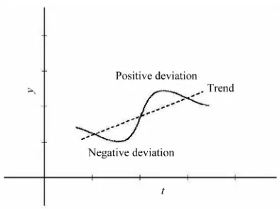
The trend of the time series is usually rough, it is not easy to recognize cyclic regularity. It needs a work of cleaning the raw data, firstly to eliminate those compo- nents that have a cyclic explanation as purely seasonal (for example the decline of industrial production in Au- gust) or accidental (as monthly variations of production caused by the different number of days working), and then also to eliminate patterns requiring a special “ad hoc” explanation, determined by important but unique events, as the effects of war, natural disasters [8,9]. The relationship between cycle and growth is a phenomenon coexisting in the representation that the empirical data provide. The majority of economists decided to solve the problem by making a clear separation of the two phe- nomena. The statistical methods used for this purpose differ in details, but in essence all consist in the evalua- tion of a trend, which should give an account of growth, and in the calculation of variances, that the considered time series show against the trend. An example, with a linear trend, is shown in Figure 2.
A substantially always increasing trend can be de- composed into two components: one showing a uniform growth for a long period of time and the other that in- stead oscillates, assuming positive or negative values in relation on whether of the considered variable overtakes the long term trend. Normally it is assumed that the trend represents the performance of system equilibrium and that cyclical deviations are due to deviations. The trend calculation is of necessity made on the basis of data of the past. But the present and the future may have very different characteristics from those of the past, especially if there are modifications of structural character, which is more probable as longer is the period of data observation [10].
Figure 2. Possible variations of a linear trend.
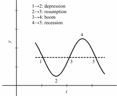
Looking at the profile of the deviations, the identifi- cation of the phases, that usually describe the cycle, be- comes easy: depression, resumption, boom, recession (Figure 3).
The amplitude of booms and depression of historical cycles had not always comparable size, so as their dura- tion was also highly variable. Therefore, some modern theorists begun to doubt the very existence of phenomena, that can be properly called cyclic [11]. Every historical cycle has its own characteristics because it takes place in different and changing socio-economic situations and is influenced by a different measure extent with endoge- nous (economic) and external (non-economic) factors [12-14]. The various indicators begin to move with greater velocity, the recovery spreads and becomes boom. It grows the production, sales, employment, real income, used production capacities, applications for raw materials and finished products, the quantity of money, its velocity of circulation, the amount of credit and loans to economy. However the boom does not last indefinitely, economic activity first begins to decelerate and then to contract.
3. Theoretical Explanations of Cycles
The reflection on the causes and mechanisms that gener- ate cyclic movements has a long history. Many of the theories of the cycle, that dominate the scene, have still now their antecedents in formulations which have ap- peared in the last century or the beginning of it. The fol- lowing treatments have benefited of a more rigorous analytical framework and a much larger amount of em- pirical knowledge.
[image:2.595.58.290.85.251.2]Figure 3. The various levels of a displacement by a trend.
much in exalting the phases of expansion and in aggra- vating that of contraction.
Later, John Stuart Mill pointed out the influence of speculation and the forecast errors of the operators that caused irrational fluctuations in the demand for credit, which, consequently, had the effect of enhancing the cyclic phenomena. At the beginning of the last century, the different theories explained the crisis in terms of un- der-consumption and savings excess [17].
It has seen that, in the case of damped oscillations, the permanence of the cycle time can be ensured by a suc- cession of irregular, random nature shocks. Theories based on the interaction between multiplier and accel- erator did not give exclusive importance on this fact [18]. On the other hand, the empirical investigations seem to suggest that the values of the parameters of the model are such as to give rise to a solution of “explosive” type, i.e. to oscillations or amplified in exponential growth. The most well-known theories have recognized this pecu- liarity, but have introduced upper and lower limits, which block the divergent trends of the system bouncing in the opposite directions [19].
Explosives trends occur at high values of the accelera- tor. With this increase in demand (exogenous), it follows a significant increase in investment and thus a rapid growth. The boom is self-fueled and the system is pushed towards the upper limit by full capacity utilization (espe- cially in sectors producing capital goods) or by the full employment of labor (with the required characteristics). The introduction of lower and upper limits allowed for a greater realism of the theory and has eliminated some important deficiencies. Richard M. Goodwin introduced the ideas of ceilings and floors [20], John R. Hicks an exogenous trend of growth for individual investments [21]. The introduction of lower and upper limits made non-linear the original model; the accelerator does not work as before when limits are reached. This is the ad- vantage of the model, but also a limit, because at linear
The new model was utilized at today at scale length of order of nanometers. But the de Broglie thermal wave- length refers to the dual nature of reality. Associating the wavelength to the impulse through the de Broglie re- lation, it is possible to define a thermal wavelength t for every object at macrolevel via the relation:
3 t h mk T
B (1)
In Equation (1), h is the Planck constant, kB the Bolt- zmann’s constant, m and T mass and temperature of the considered system respectively. With this gauge factor it is so possible to study the dynamics of reality processes presenting oscillations in time, so as characteristics of diffusivity in time.
The model offers the analytical formulation of the most important quantities related to the dynamics of a generic process, i.e.:
a) The velocities correlation function:
0 T t v v (2)
at temperature T, from which the velocity v(t) is obtain- able;
b) The mean squared deviation of position:
22 0
R t R t R (3)
from which the position vector at the time t is obtainable;
R t
c) The time-dependent diffusion D(t) of the system:
2
1 2 d d
D t R t t (4) Equations (2)-(4) are fundamental in deducing the most important characteristics concerning the transport phenomena of processes.
The roots of the model lie in the linear response theory and follow the standard time-dependent approach; the conductivity
is in general a complex function of the frequency and can be deduced from linear re- sponse theory. The model is based on a complete Fourier transform of the frequency-dependent complex conduc- tivity
of the system; this is in general a complex function of the frequency , which can be deduced from linear response theory (Green-Kubo formula):
2
0d e 0 d 0
i t
e V t t i
v v (5)velocities correlation function
0T inside the integral. The presence of an integration from 0 to is however a problem for the analytical inversion, but it can be overcame evaluating the integral on the entire time axis (, +). Considering the real part of the complex conductivity in Equation (5), the extension to the entire time axis is possible and a complete Fourier transform can be performed, obtaining directly real velocities. The integral can be resolved in the complex plane considering a Cauchy integration; as a result, the velocities correla- tion function can be evaluated exactly by the residue theorem [25]. After this step, it is possible to obtain the analytical form of the mean square deviation of position (Equation (3)) and of the diffusion coefficient D(t) (Equation (4)).
t
v v
The deduced results are, with xt:
0 exp
cos R 2 1 R sin R 2
t KT m x 2
x x
v v
(6)
2 2
0
2 1 sin 2 exp
cos 2 exp 2 1
R R
R
R t KT m x x
x x
2
(7)
2
2 4 R sin R 2 exp 2
D t KT m x x
(8) Equations (6)-(8) are related to a first model constant
2 2 0
4 1
R
; R is a real non-negative number. In the same way the model contains three analytical rela- tions related to the second model constant
2 2 0
1 4
I
; I
0,1 and real. One of the most interesting peculiarities of the model is the “time do- main” used approach, not previously found in such a contest, contrarily to the existing theoretical approaches of literature, which are “frequency domain” treatments and/or numerical methods [22-24].The model was tested with the most utilized nanoma- terials at today and describes transport properties of nano- and bio-materials [26-33], including previous im- portant models [34] and offering new interesting peculi- arities, still not experimentally found.
The analytical form of previous cited relations is com- posed by a superposition of exponentials and/or products among exponentials and sinusoidal (cosinusoidal) func- tions, giving rise to trends as indicated in Figures 4-6.
[image:4.595.307.540.83.508.2]The model is so related to variables as the temperature, the energy and the mass, the weight of the various states (at quantum level), which, “mutatis mutandis”, are very important in a lot of economic processes too, from eco- nomic geography and gravity models for economy, to economic behaviours treated with game theory [35], eco-
Figure 4. Velocities correlation functionvs t for two values of the parameter of the model R
2 2 0
4 1
. We
note clear damped oscillations in time [22-24]. R10 →
[image:4.595.320.533.84.202.2]red line; αR = 30 → green line.
Figure 5. Positive and negative deviation by a linear trend (represented in this case by t-axis) for some values of the parameter of the model I
2 2 0
1 4 [22-24]. αI = 0.1
→ red line; αI = 0.5 → blue line; αI = 0.9 → green line.
Figure 6. Behaviour of the diffusion D for I varying in
its definition interval [22-24], with τ = 10−12 s. Dots with
error bars represent experimental data. αI = 0.25 → red line;
αI = 0.75 → blue line; αI = 0.85 → green line; αI = 0.95 →
violet line.
nomic analogies to thermodynamics and chaos in busi- ness cycle theories [36,37].
[image:4.595.318.528.444.551.2]economic peculiarities.
5. Conclusion
The strength of the new derived model consists of its ability to fit very well experimental data, accommodating not completely understood behaviours and including pre- vious models, like the Smith model. The possibility to work at macrolevel through the use of the gauge factor (1) allows interesting applications in any sector in which velocities, distancies, oscillations and diffusion are in- volved. The started tests with economic data are giving favorable evidence of an interesting assistance of this model in the interpretation and comprehension of many phenomena at economic level.
REFERENCES
[1] G. Dosi and R. R. Nelson, “An Introduction to Evolu- tionary Theories in Economics,” Journal of Evolutionary Economics, Vol. 4, No. 3, 1994, pp. 153-172.
doi:10.1007/BF01236366
[2] J. T. Cuddington and C. M. Urzúa, “Trends and Cycles in the Net Barter Terms of Trade: A New Approach,” Eco- nomic Journal, Vol. 99, No. 396, 1989, pp. 426-442. doi:10.2307/2234034
[3] P. Di Sia, “Nature and Development of Econophysics: A Short Report,” Theoretical Economics Letters, Vol. 2, No. 2, 2012, pp. 183-185. doi:10.4236/tel.2012.22032
[4] “Measuring the Economy, a Primer on GDP and the Na- tional Income and Product Accounts,” 2007.
www.bea.gov
[5] http://www.hm-treasury.gov.uk/data_gdp_backgd.htm
[6] http://it.wikipedia.org/wiki/File:GDP_EU_TOP_5.svg
[7] M. Hallet, “Economic Cycles and Development Aid: What Is the Evidence from the Past?” European Commis- sion, Directorate-General for Economic and Financial Affairs, Issue 5, 2009.
[8] C. Cohen and E. D. Werker, “The Political Economy of ‘Natural’ Disasters,” Journal of Conflict Resolution, Vol. 52, No. 6, 2008, pp. 795-819.
doi:10.1177/0022002708322157
[9] D. Bergholt and P. Lujala, “Climate-Related Natural Dis- asters, Economic Growth, and Armed Civil Conflict,”
Journal of Peace Research, Vol. 49, No. 1, 2012, pp. 147-162. doi:10.1177/0022343311426167
[10] V. Zarnowitz and A. Ozyildirim, “Time Series Decompo- sition and Measurement of Business Cycles, Trends and Growth Cycles,” Journal of Monetary Economics, Vol.
Edition, Wiley, New York, 2012.
[14] T. Todorova, “Problems Book to Accompany Mathe- matics for Economists,” John Wiley & Sons, Inc., New York, 2012.
[15] A. M. Andreades, “History of the Bank of England,” 4th Edition, Frank Cass & Co. Ltd., London, 1966.
[16] J. Francis, “History of the Bank of England, Its Times and Traditions, from 1694 to 1844,” Banker’s Magazine, New York, 1862.
[17] D. F. Thompson, “John Stuart Mill and Representative Go- vernment,” Princeton University Press, Princeton, 1976.
[18] C. L. Evans and D. A. Marshall, “Fundamental Economic Shocks and the Macroeconomy,” Journal of Money, Cre- dit and Banking, Vol. 41, No. 8, 2009, pp. 1515-1555. doi:10.1111/j.1538-4616.2009.00271.x
[19] W. Semmler, “On Nonlinear Theories of Economic Cy- cles and the Persistence of Business Cycles,” Mathema- tical Social Sciences, Vol. 12, No. 1, 1986, pp. 47-76.
doi:10.1016/0165-4896(86)90047-8
[20] V. Velupillai, “Richard Goodwin: 1913-1996,” Economic Journal, Vol. 108, No. 450, 1998, pp. 1436-1449. doi:10.1111/1468-0297.00351
[21] J. R. Hicks, “Classics and Moderns: Vol. III of Collected Essays in Economic Theory,” Basil Blackwell, Oxford, 1983.
[22] P. Di Sia, “Classical and Quantum Transport Processes in Nano-Bio-Structures: A New Theoretical Model and Ap- plications,” PhD Thesis, Verona University, 2011.
[23] P. Di Sia, “An Analytical transport Model for Nanomate- rials,” Journal of Computational and Theoretical Nano- science, Vol. 8, No. 1, 2011, pp. 84-89.
doi:10.1166/jctn.2011.1663
[24] P. Di Sia, “An Analytical Transport Model for Nanomate- rials: The Quantum Version,” Journal of Computational and Theoretical Nanoscience, Vol. 9, No. 1, 2012, pp. 31- 34. doi:10.1166/jctn.2012.1992
[25] W. Rudin, “Real and Complex Analysis,” McGraw-Hill International Editions: Mathematics Series, McGraw-Hill Publishing Co., 1987.
[26] P. Di Sia, “New Theoretical Results for High Diffusive Nanosensors Based on ZnO Oxides,” Sensors and Trans- ducers Journal, Vol. 122, No. 1, 2010, p. 1.
[27] P. Di Sia, “Oscillating Velocity and Enhanced Diffusivity of Nanosystems from a New Quantum Transport Model,”
Journal of Nano Research, Vol. 16, 2011, pp. 49-54. doi:10.4028/www.scientific.net/JNanoR.16.49
doi:10.4028/www.scientific.net/JNanoR.20.143
[29] P. Di Sia, “Nanotechnology between Classical and Quan- tum Scale: Application of Anew Interesting Analytical Model,” Applied Surface Science, Vol. 5, No. 1, 2012, p. 1.
[30] P. Di Sia, “About the Influence of Temperature in Single- Walled Carbon Nanotubes: Details from a New Drude- Lorentz-Like Model,” Applied Surface Science, Vol. 275, 2013, pp. 384-388. doi:10.1016/j.apsusc.2012.10.132
[31] P. Di Sia, “A New Theoretical Model for the Dynamical Analysis of Nano-Bio-Structures,” Advances in Nano Research, Vol. 1, No. 1, 2013, p. 1.
[32] P. Di Sia, “Characteristics in Diffusion for High-Effi- ciency Photovoltaics Nanomaterials: An Interesting Ana- lysis,” Journal of Green Science and Technology, 2013, in press.
[33] P. Di Sia, “A New Drude-Lorentz-Like Model for
Rela-tivistic Particles,” Accepted for “3rd International Con- ference on Theoretical Physics, Theoretical Physics and Its Application, Moscow, 24-28 June 2013.
[34] N. V. Smith, “Classical Generalization of the Drude For- mula for the Optical Conductivity,” Physical Review, Vol. 64, No. 15, 2001, Article ID: 155106.
doi:10.1103/PhysRevB.64.155106
[35] J. von Neumann and O. Morgenstern, “Theory of Games and Economic Behavior,” 60th-Anniversary Edition, Princeton University Press, Princeton, 2004.
[36] W. M. Saslow, “An Economic Analogy to Thermodyna- mics,” American Journal of Physics, Vol. 67, No. 12, 1999, p. 1239. doi:10.1119/1.19110
![Figure 5. Positive and negative deviation by a linear trend (represented in this case by parameter of the model t-axis) for some values of the I14 220 [22-24]](https://thumb-us.123doks.com/thumbv2/123dok_us/7795838.728148/4.595.318.528.444.551/figure-positive-negative-deviation-linear-represented-parameter-values.webp)
