What said the economic theory about Portugal Another approach

(1)

What said the economic theory about

Portugal. Another approach

Martinho, Vítor João Pereira Domingues

Escola Superior Agrária, Instituto Politécnico de Viseu

2011

Online at

https://mpra.ub.uni-muenchen.de/33022/

(2)

1 WHAT SAID THE ECONOMIC THEORY ABOUT PORTUGAL.

ANOTHER APPROACH

Vitor João Pereira Domingues Martinho

Unidade de I&D do Instituto Politécnico de Viseu Av. Cor. José Maria Vale de Andrade

Campus Politécnico 3504 - 510 Viseu

(PORTUGAL)

e-mail: vdmartinho@esav.ipv.pt

ABSTRACT

With this work we try to analyse the agglomeration process in the Portuguese regions, using the New Economic Geography models. This work aims to test, also, the Verdoorn Law, with the alternative specifications of (1)Kaldor (1966), for the 28 NUTS III Portuguese in the period 1995 to 1999. It is intended to test the alternative interpretation of (2)Rowthorn (1975). With this study we want, also, to test the Verdoorn´s Law at a regional and a sectoral levels (NUTs II) for the period 1995-1999. The importance of some additional variables in the original specification of Verdoorn´s Law is yet tested, such as, trade flows, capital accumulation and labour concentration. This study analyses, also, through cross-section estimation methods, the influence of spatial effects in productivity in the NUTs III economic sectors of mainland Portugal from 1995 to 1999, considering the Verdoorn relationship. The aim of this paper is, yet, to present a contribution, with panel data, to the analysis of absolute convergence and conditional of the sectoral productivity at regional level (from 1995 to 1999). The structural variables used in the analysis of conditional convergence is the ratio of capital/output, the flow of goods/output and location ratio.

Keywords: new economic geography; Verdoorn law; convergence; cross-section and panel data; Portuguese regions.

1. INTRODUCTION

Kaldor rediscovered the Verdoorn law in 1966 and since then this Law has been tested in several ways, using specifications, samples and different periods. However, the conclusions drawn differ, some of them rejecting the Law of Verdoorn and other supporting its validity. (3)Kaldor (1966, 1967) in his attempt to explain the causes of the low rate of growth in the UK, reconsidering and empirically investigating Verdoorn's Law, found that there is a strong positive relationship between the growth of labor productivity (p) and output (q), i.e. p = f (q). Or alternatively between employment growth (e) and the growth of output, ie, e = f (q). Another interpretation of Verdoorn's Law, as an alternative to the Kaldor, is presented by (4)Rowthorn (1975, 1979). Rowthorn argues that the most appropriate specification of Verdoorn's Law is the ratio of growth of output (q) and the growth of labor productivity (p) with employment growth (e), i.e., q = f (e) and p = f (e), respectively (as noted above, the exogenous variable in this case is employment). On the other hand, Rowthorn believes that the empirical work of Kaldor (1966) for the period 1953-54 to 1963-64 and the (5)Cripps and Tarling (1973) for the period 1951 to 1965 that confirm Kaldor's Law, not can be accepted since they are based on small samples of countries, where extreme cases end up like Japan have great influence on overall results.

Although the agglomeration process have appeared more associated with economic geography, it is however noted that it is based, as the polarization, the earlier ideas of (6)Myrdal (1957) and (7)Hirschman (1958), pioneers of the processes of regional growth with characteristics cumulative. The work developed at the level of economic geography, traditional and recent attempt to explain the location of economic activities based on spatial factors. The liberal economic policies, international economic integration and technological progress have created, however, new challenges that promote agglomeration (8)(Jovanovic, 2000). So, have been developed new tools for economic geography, such as increasing returns, productive linkages, the multiple equilibria (with the centripetal forces in favor of agglomeration and centrifugal against agglomeration) and imperfect competition. These contributions have allowed some innovations in modeling the processes of agglomeration, which has become treatable by economists, a large number of issues. In particular the inclusion of increasing returns in the analytical models, which led to the call of increasing returns revolution in economics (9)(Fujita et al., 2000). (10-12)Krugman (1994, 1995 and 1998) has been the central figure in these developments. (13)Fujita (1988), (14)Fujita et al. (1996) and (15)Venables (1996), in turn, have been leaders in the development and exploration of the implications of economic models of location, based on increasing returns. These developments have helped to explain the clustering and "clustering" of companies and industries.

(3)

2

differences. For example, the authors associated with the Neoclassical theory, as (16)Solow (1956), consider that the tendency is, for the labor mobility, to alleviate, in the medium and long term, the regional disparities. This, because these authors consider the mobility of factors as a function of wages and the supply of resources as exogenous. Thus, what determines the mobility factor is their compensation. In another context, it appears that the current trend of several economic theories is to consider that the labor mobility accentuates regional disparities. Even writers in the line of neoclassical theory, as (17)Barro and Sala-i-Martin (1991), associated with endogenous growth theory, now admit that the mobility of labor reacts to processes of convergence and reduce regional disparities, but only if some conditions are met. That is, left to disappear the idea of absolute convergence for the same "steady state" of neoclassical influence, to a perspective of conditional convergence for differents "steady states".

2. THE MODELS

The models of the keynesian and convergence theories and of ther new economic geography are developed in several works like (18-20)Martinho (2011a, 2011b and 2011c).

3. DATA ANALYSIS

Considering the variables on the models, referred previously, and the availability of statistical information, we used data for the period from 1995 to 1999, disaggregated at regional level, obtained from the INE (National Accounts 2003).

4. EMPIRICAL EVIDENCE OF THE VERDOORN'S LAW

[image:3.595.82.518.383.758.2]

At Table 1, with results of estimations presented for each of the sectors and in the period 1995 to 1999, to stress that the industry has the greatest increasing returns to scale (9.091), followed by services (1.996).

Table 1: Analysis of economies of scale through the equation Verdoorn, Kaldor and Rowthorn, for each of the economic sectors and NUTS III of Portugal, for the period 1995 to 1999

Agriculture

Constant Coefficient DW R2 G.L. E.E. (1/(1-b)) Verdoorn(1) 0.010

(0.282)

0.053

(0.667) 0.542 1.690 23

---

Verdoorn

i i a bq

p 

0.023* (3.613)

1.105*

(17.910) 1.959 0.745 110

Kaldor

i i c dq

e  

-0.023* (-3.613)

-0.105**

(-1.707) 1.959 0.026 110

Rowthorn1

i

i e

p 11

-0.032* (-5.768)

-1.178*

(-9.524) 1.713 0.452 110

Rowthorn2

i

i e

q  2 2

-0.032* (-5.768)

-0.178

(-1.441) 1.713 0.019 110

Industry

(0.319)

0.053

(0.673) 0.195 2.380 23

9.091

Verdoorn -0.014*

(-2.993)

0.890*

(18.138) 2.253 0.749 110

Kaldor 0.014*

(2.993)

0.110*

(2.236) 2.253 0.044 110

Rowthorn1 0.053*

(6.739)

-0.617*

(-3.481) 2.069 0.099 110

(6.739)

0.383*

(2.162) 2.069 0.041 110

Services

(0.306)

0.096*

(8.009) 0.773 2.492 23

1.996

Verdoorn 0.007

(1.098)

0.499*

(6.362) 2.046 0.269 110

Kaldor -0.007

(-1.098)

0.502*

(6.399) 2.046 0.271 110

(19.382)

-0.432*

(-5.254) 1.993 0.201 110

(19.382)

0.568*

(6.895) 1.993 0.302 110

All Sectors

(4)

3

Verdoorn(1) 0.007

(0.188)

0.090*

(2.524) 0.203 2.588 23

6.711

Verdoorn -0.015*

(-3.245)

0.851*

(13.151) 2.185 0.611 110

Kaldor 0.015*

(3.245)

0.149*

(2.308) 2.185 0.046 110

(13.017)

-0.734*

(-5.499) 2.092 0.216 110

(13.017)

0.266**

(1.989) 2.092 0.035 110

Note: (1) cross-section Estimation * Coefficient statistically significant at 5%, ** Coefficient statistically significant at 10%, GL, Degrees of freedom; EE, Economies of scale.

Analyzing the coefficients of each of the estimated equations with the two estimation methods considered (Table 2), to point out, now and in general, the values obtained with both methods have some similarities. For agriculture, it appears that the Verdoorn coefficient has an elasticity outside acceptable limits, since it is above unity.

[image:4.595.83.515.71.165.2]

At the industry level Verdoorn coefficient (with an elasticity between 0.957 and 0.964, respectively, for the method of fixed effects and random effects) indicates the existence of strong increasing returns to scale, as expected, in the face of that by Kaldor, the industry is the engine of growth showing strong gains in productivity.

Table 2: Analysis of sectoral economies of scale in five NUTS II of Portugal Continental, for the period 1995-1999

Agriculture

M.E. Const. qi Ci/Qi Fi/Qik Ei/En DW R2 G.L.

Verdoorn

DIF 1.112* (10.961)

0.066 (0.177)

-0.153* (-2.283)

-0.717

(-0.295) 1.901 0.945 11 GLS 0.483*

(2.597)

1.117* (14.538)

-0.668 (-1.560)

-0.182* (-3.594)

0.065

(0.152) 2.501 0.945 9

Industry

M.E. Const. qi Ci/Qi Fi/Qik Ei/En DW R 2

G.L.

Verdoorn

DIF 0.957* (5.425)

0.213* (2.303)

-0.001 (-0.041)

-4.787*

(-2.506) 2.195 0.930 11 GLS -0.089

(-0.591)

0.964* (3.620)

0.217 (1.558)

-0.023 (-0.515)

0.042

(0.135) 2.818 0.909 9

Services

G.L.

Verdoorn

DIF 1.021* _(5.430) -0.116* _(-2.587) -0.020 _(-0.856) -5.458** _(-1.895) 1.369 0.846 11 GLS -1.590

(-0.734)

1.084* (5.577)

-0.106* (-2.319)

-0.020 (-0.815)

-5.985**

(-2.063) 1.629 0.717 9

All Sectors

G.L.

Verdoorn

DIF 0.905* (4.298)

-0.342* (-4.872)

-0.090* (-4.430)

-3.102*

(-2.178) 1.402 0.919 11 GLS 1.559

(1.675)

0.859* (3.776)

-0.371* (-4.665)

-0.096* (-4.404)

-3.158*

(-2.098) 1.459 0.912 9

Note: * Coefficient statistically significant at 5%, ** Coefficient statistically significant at the 10% ME, estimation method, Const., Constant; Coef., Coefficient, GL, degrees of freedom; DIF method of estimation with fixed effects and variables in differences; GLS method of estimation with random effects; C/Q, capital accumulation; F/Q, trade flow; E/E labor concentration.

In the services the Verdoorn coefficient, although statistical significance is greater than one. For the total regions, the Verdoorn equation presents results that confirm the existence of strong growing economies to scale, with additional variables to show statistical significance.

In a general analysis of Table 2, we verified the presence of strong economies of scale in the industry, confirming Kaldor's theory that this is the only sector with substantial gains in production efficiency.

This part of the study will examine the procedures of specification by (21)Florax e al. (2003) and will firstly examine through OLS estimates, the relevance of proceeding with estimate models with spatial lag and spatial error components with recourse to LM specification tests.

The results concerning the OLS estimates of the Verdoorn’s equation, without spatial variables)

(5)

4

Table 3: OLS cross-section estimates of Verdoorn’s equation with spatial specification tests (1995-1999)

Equation:

p

_it









q

_it





_it

Con. Coef. JB BP KB M’I LMl LMRl LMe LMRe R2 N.O.

Agriculture 0.013*

(3.042) 0.854*

(9.279) 1.978 5.153* 5.452* 0.331* 0.416 7.111* 8.774* 15.469* 0.759 28

Industry -0.029*

(-3.675) 1.032*

(9.250) 3.380 2.511 1.532 -0.037 1.122 2.317 0.109 1.304 0.758 28

Services 0.033*

(3.971) 0.169

(1.601) 1.391 1.638 1.697 0.212* 4.749* 1.987 3.607* 0.846 0.055 28

Total of sectors

0.002 (0.411)

0.659*

(8.874) 1.585 5.174* 4.027* 0.030 0.008 0.087 0.069 0.149 0.742 28 Note: JB, Jarque-Bera test to establish parameters; BP, Breusch-Pagan test for heteroskedasticity; KB, Koenker-Bassett test for heteroskedasticity: M’I, Moran’s I statistics for spatial autocorrelation; LMl, LM test for

spatial lag component; LMRl, robust LM test for spatial lag component; LMe, LM test for spatial error

component; LMRe, robust LM test for spatial error component;R2, coefficient of adjusted determination; N.O.,

number of observations; *, statistically significant for 5%

From the table 3 the existence of growing scaled income in agriculture and in the total of all sectors is confirmed. Industry shows itself to be a sector with very strong growing scaled income, since,

despite Verdoorn’s coefficient being highly exaggerated it is very close to unity and when the null

hypothesis is tested as



=1, a t-statistic of 0.287 is obtained. As it is a highly reduced value, it is

accepted that industry is subject to strong scaled income.

The results for ML estimates with spatial effects for agriculture and services are presented in table 4.

Table 4: Resultsfor ML estimates for Verdoorn’s equation with spatial effects (1995-1999)

Constant Coefficient Coefficient(S)

Breusch-Pagan R

2 _{N.Observations}

Agriculture 0.016*

(1.961)

0.988* (14.291)

0.698*

(4.665) 4.246* 0.852 28

Services 0.011

(0.945)

0.134 (1.464)

0.545*

(2.755) 3.050** 0.269 28

Note: Coefficient(S), spatial coefficient for the spatial error model for agriculture and the spatial lag model for services; *, statistically significant to 5%; **, statistically significant to 10%.

Only in agriculture the Verdoorn’s coefficient improves with the consideration of spatial effects,

since it goes from 0.854 to 0.988.

5. EMPIRICAL EVIDENCE OF THE NEW ECONOMIC GEOGRAPHY

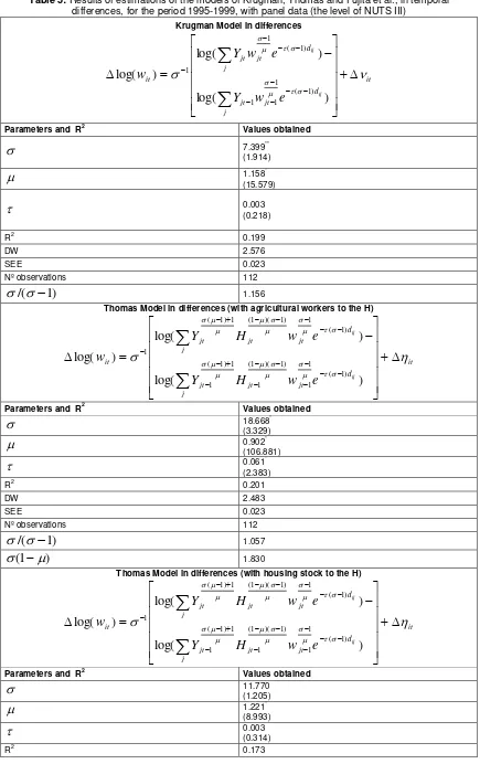
According to Table 5, with the results obtained in the estimations for the period 1995 to 1999, although the estimation results with the model equation of Thomas (with agricultural employment as a

force anti- agglomeration) are more satisfying, considering the parameter values

_

less than unity as

would be expected in view of economic theory. Note that when considering the stock of housing as centrifugal force, although the results show evidence of greater economies of scale (as noted by the data analysis, because the close relationship between this variable and nominal wages) are statistically less

satisfactory. There is also that



_/(





₁

₎

values are always higher than unity, is confirmed also for this

period the existence of increasing returns to scale, although with a moderate size, given the value

)

1 (







, i.e. 1.830, in the model Thomas. Since as noted above, when



₍

₁





₎



₁

increasing

returns to scale are sufficiently weak or the fraction of the manufactured goods sector is sufficiently low and the range of possible equilibria depends on the costs of transportation. Should be noted that the

parameter



is not statistical significance in Krugman model and present a very low value in the model of

(6)

[image:6.595.81.516.76.768.2]

5

Table 5: Results of estimations of the models of Krugman, Thomas and Fujita et al., in temporal differences, for the period 1995-1999, with panel data (the level of NUTS III)

Krugman Model in differences

it j d jt jt j d jt jt it ij ij

e

w

Y

e

w

Y

w





       

























        

)

log(

)

log(

)

log(

) 1 ( 1 1 1 ) 1 ( 1 1

Parameters and R2 Values obtained



7.399**

(1.914)



1.158*

(15.579)



0.003

(0.218)

R2 0.199

DW 2.576

SEE 0.023

Nº observations 112

)

1 /(







1.156

Thomas Model in differences (with agricultural workers to the H)

it j d jt jt jt j d jt jt jt it ij ij

e

w

H

Y

e

w

H

Y

w





                   

























                 

)

log(

)

log(

)

log(

) 1 ( 1 1 ) 1 )( 1 ( 1 1 ) 1 ( 1 ) 1 ( 1 ) 1 )( 1 ( 1 ) 1 ( 1



18.668*

(3.329)



0.902*

(106.881)



0.061*

(2.383)

R2 0.201

DW 2.483

SEE 0.023

)

1 /(







1.057

)

1 (







1.830

Thomas Model in differences (with housing stock to the H)

it j d jt jt jt j d jt jt jt it ij ij

e

w

H

Y

e

w

H

Y

w





                   

























                 

)

log(

)

log(

)

log(

) 1 ( 1 1 ) 1 )( 1 ( 1 1 ) 1 ( 1 ) 1 ( 1 ) 1 )( 1 ( 1 ) 1 ( 1



11.770

(1.205)



1.221*

(8.993)



0.003

(0.314)

(7)

6

DW 2.535

SEE 0.024

Fujita et al. Model in differences

it

j

ijt jt jt j

ijt jt jt it

T

w

Y

T

w

Y

w





 

   

























   

 

  



)

log(

)

log(

)

log(

) 1 ( 1 1

1 1

) 1 ( 1

1



5.482*

(4.399)



1.159*

(14.741)

R2 0.177

DW 2.594

SEE 0.023

)

1 /(







1.223

Note: Figures in brackets represent the t-statistic. * Coefficients significant to 5%. ** Coefficients significant acct for 10%.

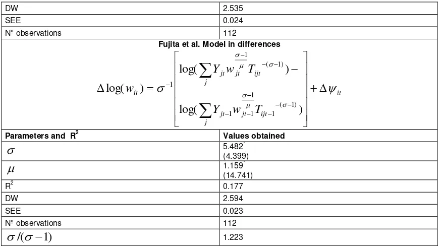
6. EMPIRICAL EVIDENCE OF ABSOLUTE CONVERGENCE WITH PANEL DATA

Are presented subsequently in Table 6 the results of the absolute convergence of output per worker, obtained in the panel estimations for each of the sectors and all sectors, now at the level of NUTS III during the period 1995 to 1999.

[image:7.595.80.516.69.314.2]

The results of convergence are statistically satisfactory for all sectors and for the total economy of the NUTS III.

Table 6: Analysis of convergence in productivity for each of the economic sectors at the level of NUTS III of Portugal, for the period 1995 to 1999

Agriculture

Method Const. Coef. T.C. DW R2 G.L.

Pooling 0.017 (0.086)

-0.003

(-0.146) -0.003 2.348 0.000 110 LSDV -0.938*

(-9.041) -2.781 2.279 0.529 83 GLS -0.219*

(-3.633)

0.024*

(3.443) 0.024 1.315 0.097 110

Industry

Pooling 0.770* (4.200)

-0.076*

(-4.017) -0.079 1.899 0.128 110 LSDV -0.511*

(-7.784) -0.715 2.555 0.608 83 GLS 0.875*

(4.154)

-0.086*

(-3.994) -0.090 2.062 0.127 110

Services

Pooling 0.258 (1.599)

-0.022

(-1.314) -0.022 1.955 0.016 110 LSDV -0.166*

(-5.790) -0.182 2.665 0.382 83 GLS 0.089

(0.632)

-0.004

(-0.303) -0.004 1.868 0.001 110

All sectors

“Pooling” 0.094 _(0.833) -0.005 _(-0.445) -0.005 2.234 0.002 110

LSDV -0.156*

(-3.419) -0.170 2.664 0.311 83 GLS 0.079

(0.750)

-0.004

(-0.337) -0.004 2.169 0.001 110

(8)

7

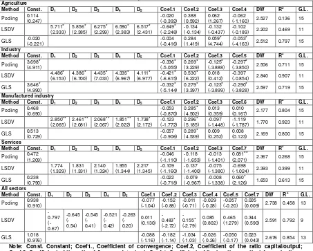
7. EMPIRICAL EVIDENCE OF CONDITIONAL CONVERGENCE WITH PANEL DATA

This part of the work aims to analyze the conditional convergence of labor productivity sectors (using as a "proxy" output per worker) between the different NUTS II of Portugal, from 1995 to 1999.

[image:8.595.72.525.215.578.2]

Given these limitations and the availability of data, it was estimated in this part of the work the equation of convergence introducing some structural variables, namely, the ratio of gross fixed capital/output (such as "proxy" for the accumulation of capital/output ), the flow ratio of goods/output (as a "proxy" for transport costs) and the location quotient (calculated as the ratio between the number of regional employees in a given sector and the number of national employees in this sector on the ratio between the number regional employment and the number of national employees) ((22) Sala-i-Martin, 1996).

Table 7: Analysis of conditional convergence in productivity for each of the sectors at NUTS II of Portugal, for the period 1995 to 1999

Agriculture

Method Const. D1 D2 D3 D4 D5 Coef.1 Coef.2 Coef.3 Coef.4 DW R2 G.L.

Pooling 0.114 (0.247) -0.020 (-0.392) 0.388 (0.592) 0.062 (1.267) -0.062

(-1.160) 2.527 0.136 15 LSDV 5.711*

(2.333) 5.856* (2.385) 6.275* (2.299) 6.580* (2.383) 6.517* (2.431) -0.649* (-2.248) -0.134 (-0.134) -0.132 (-0.437) -0.102

(-0.189) 2.202 0.469 11 GLS -0.020

(-0.221) -0.004 (-0.416) 0.284 (1.419) 0.059* (4.744) -0.053*

(-4.163) 2.512 0.797 15

Industry

Pooling 3.698* (4.911) -0.336* (-5.055) 0.269* (3.229) -0.125* (-3.888) -0.297*

(-3.850) 2.506 0.711 15 LSDV 4.486*

(6.153) 4.386* (6.700) 4.435* (7.033) 4.335* (6.967) 4.111* (6.977) -0.421* (-6.615) 0.530* (6.222) 0.018 (0.412) -0.397

(-0.854) 2.840 0.907 11 GLS 3.646*

(4.990) -0.332* (-5.144) 0.279* (3.397) -0.123* (-3.899) -0.290*

(-3.828) 2.597 0.719 15

Manufactured industry

Pooling 0.468 (0.690) -0.053 (-0.870) 0.285* (4.502) 0.013 (0.359) 0.010

(0.167) 2.177 0.804 15 LSDV 2.850**

(2.065) 2.461** (2.081) 2.068** (2.067) 1.851** (2.022) 1.738* (2.172) -0.123 (-1.772) 0.296* (5.185) -0.097 (-1.448) -1.119

(-1.787) 1.770 0.923 11 GLS 0.513

(0.729) -0.057 (-0.906) 0.289* (4.539) 0.009 (0.252) 0.008

(0.123) 2.169 0.800 15

Services

Pooling 0.472 (1.209) -0.046 (-1.110) -0.118 (-1.653) -0.013 (-1.401) 0.081**

(2.071) 2.367 0.268 15 LSDV 1.774

(1.329) 1.831 (1.331) 2.140 (1.324) 1.955 (1.344) 2.217 (1.345) -0.109 (-1.160) -0.137 (-1.400) -0.075 (-1.380) -0.698

(-1.024) 2.393 0.399 11 GLS 0.238

(0.790) -0.022 (-0.718) -0.079 (-0.967) -0.008 (-1.338) 0.060*

(2.126) 1.653 0.613 15

All sectors

Method Const. D1 D2 D3 D4 D5 Coef.1 Coef.2 Coef.3 Coef.4 Coef.5 Coef.7 DW R2 G.L.

Pooling 0.938 (0.910) -0.077 (-1.04) -0.152 (-0.88) -0.011 (-0.71) -0.029 (-0.28) -0.057 (-0.20) 0.005

(0.009) 2.738 0.458 13

LSDV -0.797 (-0.67) -0.645 (-0.54) -0.545 (-0.41) -0.521 (-0.42) -0.263 (-0.20) 0.011 (0.130) -0.483* (-2.72) -0.155* (-2.79) 0.085 (0.802) 0.465 (1.279) 0.344

(0.590) 2.591 0.792 9

GLS 1.018 (0.976) -0.088 (-1.16) -0.182 (-1.14) -1.034 (-1.03) -0.026 (-0.26) -0.050 (-0.17) 0.023

(0.043) 2.676 0.854 13 Note: Const. Constant; Coef1., Coefficient of convergence; Coef.2, Coefficient of the ratio capital/output; Coef.3, Coefficient of the ratio of flow goods/output; Coef.4, Coefficient of the location quotient for agriculture; Coef.5, Coefficient of industry location quotient; Coef.6, Coefficient of the location quotient for manufacturing; Coef.7, Coefficient quotient location of services; * Coefficient statistically significant at 5%, ** statistically significant coefficient 10%; GL, Degrees of freedom; LSDV, Method of variables with fixed effects dummies; D1 ... D5, five variables dummies corresponding to five different regions.

Therefore, the data used and the results obtained in the estimations made, if we have conditional convergence, that will be in industry.

8. CONCLUSIONS

In light of what has been said above, we can conclude the existence of agglomeration processes in Portugal (around Lisboa e Vale do Tejo) in the period 1995 to 1999, given that the transport costs are low and that there are increasing returns to scale in manufacturing in the Portuguese regions.

(9)

8

improvement have in the Verdoorn coefficient. With the cross-section estimates, it can be seen, that sector by sector the growing scaled income is much stronger in industry and weaker or non-existent in the other

sectors, just as proposed by Kaldor. With reference to spatial autocorrelation, Moran’s I value is only

statistically significant in agriculture and services.

The convergence theory is not clear about the regional tendency in Portugal, so the conclusions about the regional convergence are not consistent.

So, in this period, we can conclude that the economic theory said which in Portugal we had regional divergence around Lisbon.

9. REFERENCES

1. N. Kaldor. Causes of the Slow Rate of Economics of the UK. An Inaugural Lecture. Cambridge: Cambridge University Press, 1966.

2. R.E. Rowthorn. What Remains of Kaldor Laws? Economic Journal, 85, 10-19 (1975). 3. N. Kaldor. Strategic factors in economic development. Cornell University, Itaca, 1967. 4. R.E. Rowthorn. A note on Verdoorn´s Law. Economic Journal, Vol. 89, pp: 131-133 (1979).

5. T.F. Cripps and R.J. Tarling. Growth in advanced capitalist economies: 1950-1970. University of Cambridge, Department of Applied Economics, Occasional Paper 40, 1973.

6. G. Myrdal. Economic Theory and Under-developed Regions. Duckworth, London, 1957. 7. A. Hirschman. The Strategy of Economic Development. Yale University Press, 1958.

8. M.N. Jovanovic. M. Fujita, P. Krugman, A.J. Venables - The Spatial Economy. Economia Internazionale, Vol. LIII, nº 3, 428-431 (2000).

9. M. Fujita; P. Krugman and J.A. Venables. The Spatial Economy: Cities, Regions, and International Trade. MIT Press, Cambridge, 2000.

10. P. Krugman. Complex Landscapes in Economic Geography. The American Economic Review, Vol. 84, nº 2, 412-416 (1994).

11. P. Krugman. Development, Geography, and Economic Theory. MIT Press, Cambridge, 1995.

12. P. Krugman. Space: The Final Frontier. Journal of Economic Perspectives, Vol. 12, nº 2, 161-174 (1998).

13. M. Fujita. A monopolistic competition model of spatial agglomeration: Differentiated product approach. Regional Science and Urban Economics, 18, 87-125 (1988).

14. M. Fujita and T. Mori. The role of ports in the making of major cities: Self-agglomeration and hub-effect. Journal of Development Economics, 49, 93-120 (1996).

15. A.J. Venables. Equilibrium locations of vertically linked industries. International Economic Review, 37, 341-359 (1996).

16. R. Solow. A Contribution to the Theory of Economic Growth. Quarterly Journal of Economics (1956). 17. R. Barro and X. Sala-i-Martin. Convergence across states and regions. Brooking Papers on Economic Activity, 1, pp: 82-107 (1991).

18. V.J.P.D. Martinho. The importance of increasing returns to scale in the process of agglomeration in Portugal: A non linear empirical analysis. MPRA Paper 32204, University Library of Munich, Germany (2011a).

19. V.J.P.D. Martinho. What the keynesian theory said about Portugal?. MPRA Paper 32610, University Library of Munich, Germany (2011b).

20. V.J.P.D. Martinho. What said the neoclassical and endogenous growth theories about Portugal?. MPRA Paper 32631, University Library of Munich, Germany (2011c).

21. R.J.G.M Florax.; H. Folmer; and S.J. Rey. Specification searches in spatial econometrics: the relevance of Hendry´s methodology. ERSA Conference, Porto 2003.