Munich Personal RePEc Archive
Analytical approximation of the
transition density in a local volatility
model
Pagliarani, Stefano and Pascucci, Andrea
Università di Padova, Università di Bologna
4 May 2011
Online at
https://mpra.ub.uni-muenchen.de/31107/
Analytical approximation of the transition density
in a local volatility model
Stefano Pagliarani∗, Andrea Pascucci†
May 4, 2011
Abstract
We present a simplified approach to the analytical approximation of the transition density related to a general local volatility model. The methodology is sufficiently flexible to be extended to time-dependent coefficients, multi-dimensional stochastic volatility models, degenerate parabolic PDEs related to Asian options and also to include jumps.
1
Introduction
Analytical approximation methods in option pricing have attracted an ever increasing interest in the last years. This is due to the demand for more sophisticated pricing models, including local, stochastic volatility and/or jumps, that generally cannot be solved in closed-form: for these models, the practical issue of the implementation is striking, in particular in the calibra-tion and risk management processes that are typically very demanding and computationally time-consuming. The main advantage of the analytical ap-proaches with respect to other numerical methods, such as finite-difference and Fourier inversion, is that in general the first ones are much faster and precise, at least under certain model parameter regime. Secondly, analytic formulae retain qualitative model information and preserve an explicit de-pendence of the results on the underlying parameters.
The application of asymptotic expansions and singular perturbation meth-ods in mathematical finance has been studied by several authors: one of the first results was obtained by Whalley and Wilmott [32] in the study of transaction costs; in the seminal paper [19] Hagan and Woodward derived an asymptotic expansion formula for the implied volatility in a local volatil-ity (LV) model where the volatilvolatil-ity function can be written as the product
∗Email: [email protected], Dipartimento di Matematica, Universit`a di Padova,
Via Trieste 63, 35121 Padova, Italy
†Email: [email protected], Dipartimento di Matematica, Universit`a di Bologna,
of two independent functions of time and underlying, the prototype example being the constant elasticity of variance (CEV) model; the approximation of more general one-dimensional LV models, using different deterministic and probabilistic techniques, was studied among others by Howison [23], Wid-dicks, Duck, Andricopoulos and Newton [33], Capriotti [5], Gatheral, Hsu, Laurence, Ouyang and Wang [16], Benhamou, Gobet and Miri [3]. A fur-ther different approach based on heat kernel expansion and the parametrix method was proposed by Corielli, Foschi and Pascucci [8], Constantinescu, Costanzino, Mazzucato and Nistor [7], Cheng, Costanzino, Liechty, Mazzu-cato and Nistor [6], Kristensen and Mele [25].
Asymptotic methods for two-factor stochastic volatility models were studied by Hagan, Kumar, Lesniewski and Woodward [17] who introduced the SABR model; further improvements were proposed by Fouque, Papan-icolaou, Sircar and Solna [15], Berestycki, Busca and Florent [4], Antonelli and Scarlatti [1]. In [26] Lesniewski introduced a geometric approach to the approximation of stochastic volatility models using the heat kernel ex-pansion on a Riemann manifold: this approach was further developed by Hagan, Lesniewski and Woodward [18], Paulot [29], Taylor [31] and Henry-Labord`ere who in [20] generalized the SABR to a model with mean-reverting volatility, the so-called λ-SABR.
In this paper we are mainly concerned with one-dimensional LV models of the form
dSt=µ(t, St)dt+σ(t, St)StdWt; (1.1) we present in this simplel framework a methodology that can be applied to multi-dimensional models, jump-diffusion models and even in the case of ultraparabolic pricing equations such as PDEs for Asian options: these and other issues are covered in the forthcoming paper [14].
The starting point of our analysis is the paper by Hagan and Woodward [19]. We develop the approach in [19] and show how it can be simplified and adapted to derive an expansion directly of the density of the underlying pro-cess, with the possibility of incorporating time-dependency and even jumps. Our main result is an expansion of the transition density Γ(t, S0;T, S) of S
in (1.1) of the form
Γ(t, S0;T, S) ≈ G0(t, S0;T, S) +
N
X
n=1
JSn0G0(t, S0;T, S), N ≥1, (1.2)
where the main termG0(t, S
0;T, S) is the density in a suitable Black&Scholes
model, whileJn
S0 is a differential operator containing derivatives with respect
to the variable S0: thus the terms of the expansion (1.2) are linear
From (1.2), we can easily derive the prices and the Greeks of plain vanilla options: for instance, for a Call option with strike K and maturity T, we have
C(t, S0) =
Z
Γ(t, S0;T, S) (S−K)+dS
≈ 1 + N
X
n=1
JSn0
! Z
Γ0(t, S0;T, S) (S−K)+dS
=CBS(t, S0) +
N
X
n=1
JSn0CBS(t, S0),
whereCBSdenotes a Black&Scholes price. Formula (1.2) can also be used to
price efficiently American options and other exotic derivatives. We remark that the accuracy of the approximation is independent of the smoothness of the payoff function because the operators of the expansion act directly on the transition density of the process and not on the payoff function. Another key feature of our approach is that at any order the approximated density integrates to one (cf. Remark 2.5), thus avoiding the introduction of arbitrage opportunities: for instance, the approximated option prices verify the Put-Call parity.
Finally, the smaller the time lag T −t is, the faster the convergence of the expansion is. Thus, for longer maturities, it is advantageous to split the time interval in order to get a significant improvement of the accuracy. In Remark 2.4, we show how this can be done by using the expansion (1.2) and also in this case we find explicit formulae.
The layout of the paper is as follows. In Section 2 we present our main results and provide the full detail of the proof in a simplified setting. In Section 3 we carry the expansion out to order two (i.e. N = 2 in (1.2)) for the general LV model (1.1). The numerical Section 4 investigates the effectiveness of the approximation obtained in two relevant models: in the case of a quadratic LV model we test the expansion against standard Monte Carlo approximation; secondly, we analyze more extensively the CEV model and compare ours to the earlier approximations by Hagan and Woodward [19] and by Henry-Labord`ere [20].
2
Analytical approximation of parabolic
fundamen-tal solutions
In this section we present the approximation technique in the simplest case of a differential operator of the form
L= a(x)
2 ∂xx+∂t, (t, x)∈R
2, (2.3)
whereais a smooth function such that
a0≤a(x)≤C, x∈R,
for some positive constantsa0 and C. For simplicity of exposition, we only
consider time-independent coefficients and refer to Section 3 for the general case. By taking the Taylor expansion of a with starting point ¯x ∈ R, we
have
L=L0+
∞
X
k=1
αk(x−x¯)k∂xx (2.4)
where
L0 = α0
2 ∂xx+∂t, α0 =a(¯x), (2.5) is the 0-th order approximation of Land
αn= 1 2n!∂
n
xa(¯x), n≥1.
We denote by Γ(t, x;T, y) the fundamental solution ofL evaluated at (t, x) with pole in (T, y): from the probabilistic point of view, Γ(t, x;T, y) is the transition density of the solution to the SDE
dXt=
p
a(Xt)dWt, (2.6)
where W is a standard Wiener process: precisely, y 7→ Γ(t, x;T, y) is the density of the random variable XTt,x, where Xt,x denotes the solution of (2.6) with initial conditionXtt,x =x.
We aim to approximate Γ by an expansion of the form
Γ(t, x;T, y) =X k≥0
Gk(t, x;T, y) (2.7)
where the Gk
k≥0 is defined recursively in terms of the solutions of a
se-quence of Cauchy problems. More precisely, the leading term of the expan-sion
G0(t, x;T, y) := p 1
2πα0(T −t)
exp
− (x−y)
2
2α0(T −t)
, x, y∈R, t < T,
is the fundamental solution of L0 in (2.5). Moreover, for any (T, y) ∈ R2,
we denote byG1(·,·;T, y) the solution of the Cauchy problem
(
L0G1(t, x;T, y) +α1(x−x¯)∂xxG0(t, x;T, y) = 0, t < T, x∈R,
G1(t, x;T, y) = 0, x∈R,
(2.9) and byG2(·,·;T, y) the solution to
(
L0G2+α1(x−x¯)∂xxG1+α2(x−x¯)2∂xxG0 = 0, t < T, x∈R,
G2(t, x;T, y) = 0, x∈R.
(2.10) In general, we put
ΓN(t, x;T, y) = N
X
n=0
Gn(t, x;T, y), N ≥0,
and we define recursively the sequence (Gn)
n∈N by setting
L0Gn+ Pn k=1
αk(x−x¯)k∂xxGn−k= 0, t < T, x∈R,
Gn(t, x;T, y) = 0, x∈R.
(2.11)
Remark 2.1. The particular choice of the Cauchy problems (2.11) comes from the fact that
L0ΓN = N
X
n=0
L0Gn =
(by (2.11))
=−
N
X
n=0
n
X
k=1
αk(x−x¯)k∂xxGn−k=− N
X
k=1
αk(x−x¯)k∂xx N
X
n=k
Gn−k
=−
N
X
k=1
αk(x−x¯)k∂xxΓN−k, (2.12)
and passing to the limit as N → ∞, from (2.12) and (2.4) we get
L
∞
X
n=0
Gn= 0.
Moreover, formally we have
ΓN(T, x;T, y) =G0(T, x;T, y) =δ(x−y),
In order to compute the explicit solution to problems (2.11), we recall some properties of the Gaussian density Γ0 =G0 in (2.8). First of all, we shall use the following general reproduction (or semigroup) property of Γ0 (cf., for instance, [28]): for any t < s < T and x, y∈R, we have
Z
R
Γ0(t, x;s, η)Γ0(s, η;T, y)dη= Γ0(t, x;T, y). (2.13)
Moreover we need the following elementary lemma.
Lemma 2.2. For any x, y∈R and t < T, we have
∂yΓ0(t, x;T, y) =−∂xΓ0(t, x;T, y), (2.14)
yΓ0(t, x;T, y) =xΓ0(t, x;T, y) + (T−t)α0∂xΓ0(t, x;T, y). (2.15)
Proof. Formula (2.15) is obvious by symmetry, while formula (2.14) follows from the identity
∂xΓ0(t, x;T, y) =−
x−y
(T −t)α0
Γ0(t, x;T, y).
By Lemma 2.2, the partial derivative ∂y acts as −∂x on Γ0(t, x;T, y). Moreover, ifmx denotes the product operator
mxf =xf, (2.16)
then, for anyc∈R, the operator my+c acts as
mx+c+ (T −t)α0∂x
on Γ0(t, x;T, y). More generally, we also have
(y+c)kΓ0(t, x;T, y) =mky+cΓ0(t, x;T, y)
= (mx+c+ (T −t)α0∂x)kΓ0(t, x;T, y)
for any k∈N.
Proposition 2.3. The solution Gn of problem (2.11) is given by
Gn(t, x;T, y) =Jt,T,xn Γ0(t, x;T, y)
where Jt,T,xn is a differential operator of the form
Jn t,T,x=
3n
X
k=2
withcn,k ∈R, pk, qk ∈N such that1
2pn,k ≥n, (2.18)
and2
2pn,k+qn,k−k=n. (2.19)
The operators Jn
t,T,x in (2.17) can be computed iteratively (cf. Remark 2.4):
for instance, for n= 1,2 we have
Jt,T,x1 =α1(T−t)(x−x¯)∂x2+
α1α0
2 (T −t)
2∂3
x, (2.20)
Jt,T,x2 =α2
2 (T−t) α0(T−t) + 2(x−x¯)
2∂2
x
+ α21+α0α2
(T−t)2(x−x¯)∂x3
+
1
6(T −t)
3α
0 3α21+ 2α0α2+
1
2(T −t)
2α2
1(x−x¯)2
∂4x
+α0α
2 1
2 (T −t)
3(x−x¯)∂5
x+
α20α21
8 (T−t)
4∂6
x. (2.21)
Proof. By the standard representation formula for solutions to the non-homogeneous parabolic Cauchy problem with null final condition, we have
G1(t, x;T, y) =
Z T
t
Z
R
Γ0(t, x;s, η)α1(η−x¯)∂ηηΓ0(s, η;T, y)dηds =
(using notation (2.16))
=α1
Z T
t
Z
R
mη−x¯Γ0(t, x;s, η)∂ηηΓ0(s, η;T, y)dηds =
(by (2.15))
=α1
Z T
t
(mx−x¯+ (s−t)α0∂x)
Z
R
Γ0(t, x;s, η)∂ηηΓ0(s, η;T, y)dηds=
(by parts)
=α1
Z T
t
(mx−x¯+ (s−t)α0∂x)
Z
R
∂ηηΓ0(t, x;s, η)Γ0(s, η;T, y)dηds=
(by (2.14))
=α1
Z T
t
(mx−x¯+ (s−t)α0∂x)∂xx
Z
R
Γ0(t, x;s, η)Γ0(s, η;T, y)dηds=
1By (2.18), the approximation is better for shorter times and largern.
2By (2.19), there is a sort of parabolic homogeneity and the damping effect ofT
−t
andx
(by the reproduction property (2.13))
=α1
Z T
t
(mx−x¯+ (s−t)α0∂x)ds ∂xxΓ0(t, x;T, y).
Thus we have
Jt,T,x1 =α1
Z T
t
(mx−x¯+ (s−t)α0∂x)ds ∂xx (2.22)
and integrating inswe get (2.20). Concerning G2, we have
G2(t, x;T, y) =I1+I2
where, proceeding as before,
I1 =α2
Z T
t
Z
R
Γ0(t, x;s, η)(η−x¯)2∂ηηΓ0(s, η;T, y)dηds
=α2
Z T
t
(mx−x¯+ (s−t)α0∂x)2∂xx
Z
R
Γ0(t, x;s, η)Γ0(s, η;T, y)dηds
=α2
Z T
t
(mx−x¯+ (s−t)α0∂x)2ds ∂xxΓ0(t, x;T, y),
and
I2 =α1
Z T
t
Z
R
Γ0(t, x;s, η)(η−x¯)∂ηηG1(s, η;T, y)dηds
=α1
Z T
t
(mx−x¯+ (s−t)α0∂x)∂xx
Z
R
Γ0(t, x;s, η)Js,T,η1 Γ0(s, η;T, y)dηds
=α1
Z T
t
(mx−x¯+ (s−t)α0∂x)∂xxJes,T,x1
Z
R
Γ0(t, x;s, η)Γ0(s, η;T, y)dηds
=α1
Z T
t
(mx−x¯+ (s−t)α0∂x)∂xxJes,T,x1 dsΓ0(t, x;T, y),
with
e
Js,T,x1 =α1(T−s) (mx−x¯+ (s−t)α0∂x)∂x2+
α1α0(T−s)2
2 ∂
3
x.
In conclusion we have
Jt,T,x2 =α2
Z T
t
(mx−x¯+ (s−t)α0∂x)2ds ∂xx
+α1
Z T
t
(mx−x¯+ (s−t)α0∂x)∂xxJes,T,x1 ds.
(2.23)
Remark 2.4. The proof of Proposition 2.3 provides a constructive algorithm that can be used to compute higher order approximations iteratively. In particular this can be done by means of a symbolic computation software to get the explicit expression of the operators Jn
t,T,x in (2.17): for instance,
using Mathematica one can find the expression of Jt,T,x1 in (2.22) or Jt,T,x2
in (2.23) by writing just one line of code. Moreover, since the derivatives of the Gaussian density Γ0 can be expressed in terms of Hermite polynomials, the computation of the terms of the expansion is extremely fast.
According to (2.7), the N-th order approximation of Γ is given by
ΓN(t, x;T, y) = N
X
n=0
Gn(t, x;T, y).
By Proposition 2.3 we have
ΓN(t, x;T, y) = Γ0(t, x;T, y) +ANt,T,xΓ0(t, x;T, y), (2.24)
where Γ0 ≡G0 is the Gaussian density in (2.8) and AN
t,T,x is the differential operator
ANt,T,x= N
X
n=1
Jt,T,xn , N ≥1. (2.25)
Remark 2.5. From formula (2.24), we infer that
Z
R
ΓN(t, x;T, y)dy = (1 +AN t,T,x)
Z
R
Γ0(t, x;T, y)dy = 1.
Thus, a general property of the approximated densityΓN is that it integrates
to one.
More generally, a nice feature of the approximation formula (2.24) is thatAN
t,T,x acts as a differential operator in the variablex(starting point of the underlying stochastic process). As a consequence, the price of an option with payoff functionϕis simply given by
C(t, x) =
Z
Γ(t, x;T, y)ϕ(y)dy
≈(1 +ANt,T,x)
Z
R
Γ0(t, x;T, y)ϕ(y)dy = CBS(t, x) +ANt,T,xCBS(t, x),
where CBS denotes the option price in a Gaussian model (Black&Scholes).
The approximation formula for the density is useful to price American options and other exotic derivatives. The Greeks/sensitivities can be easily computed as well: indeed, notice that
∂xC(t, x) ≈ ∂xCBS(t, x) +∂xANt,T,xCBS(t, x)
so that the problem of the irregularity of the payoff function (typical of Monte Carlo approximation) is overcome.
Remark 2.6. Even if not stated explicitly, the approximation result of Proposition 2.3 depends on the choice of starting pointx¯of the Taylor expan-sion. With the specification x¯ =x, we get a particularly simple expression of the operators Jn
t,x,T in (2.20)-(2.21):
Jt,T,x1 =α1α0(T −t)
2
2 ∂
3
x, (2.26)
Jt,T,x2 =α2α0
2 (T −t)
2∂2
x+
α0
6 2α0α2+ 3α
2 1
(T −t)3∂x4+α
2 0α21
8 (T −t)
4∂6
x,
Jt,T,x3 =α0
3 (4α1α2+ 3α0α3)(T−t)
3∂3
x
+α0 12 6α
3
1+ 16α0α1α2+ 3α20α3(T −t)4∂x5
+α
2 0α1
12 3α
2
1+ 2α0α2(T−t)5∂x7+
α3 0α31
48 (T−t)
6∂9
x.
Other specifications of x¯ can be used to minimize the approximation error.
Remark 2.7. The approximation can be further improved by using the re-production property (2.13) and exploiting the fact that the approximation is more efficient for short maturities because of the presence of powers ofT−t
in the coefficients of the expansion. We first note that, integrating by parts and by (2.14), for Jt,T,x1 as in (2.26) we have
Z
R
Γ0(t, x;s, η) 1 +Js,T,η1 Γ0(s, η;T, y)dη=
= 1 +Js,T,x1 Z
R
Γ0(t, x;s, η)Γ0(s, η;T, y)dη =
(by the reproduction property)
= 1 +Js,T,x1 Γ0(t, x;T, y). (2.27)
Then, for any t < s < T and x, y∈R, we have
Γ(t, x;T, y) =
Z
R
Γ(t, x;s, η)Γ(s, η;T, y)dη
≈
Z
R
1 +Jt,s,x1 Γ0(t, x;s, η) 1 +Js,T,η1 Γ0(s, η;T, y)dη
= 1 +Jt,s,x1 Z
R
(by (2.27))
= 1 +Jt,s,x1 1 +Js,T,x1 Γ0(t, x;T, y).
In general, for any t < s1 <· · ·< sN < T we have
Γ(t, x;T, y)≈ 1 +Jt,s1 1,x 1 +Js11,s2,x· · · 1 +Js1N,T,xΓ0(t, x;T, y),
that is easily computable and may improve the approximation for long ma-turities.
3
Applications to local volatility models
We now consider the more general dynamics of a LV model in the risk-neutral measure
dSt=rStdt+σ(t, St)StdWt (3.28)
whereσ(t, S) is a suitably regular function such that
σ1 ≤σ(t, S)≤σ2, t >0, S >0, (3.29)
for some positive constants σ1, σ2. The pricing Cauchy problem is
(
LC(t, S) = 0, t < T, S >0, C(T, S) =ϕ(S), S >0,
where
L= σ
2(t, S)S2
2 ∂SS+rS∂S+∂t−r. (3.30) The function
u(t, x) =er(T−t)C(t, ex)
solves the parabolic Cauchy problem
(
Lu(t, x) = 0, t < T, x∈R, u(T, x) =ϕ(ex), x∈R,
where
L= a(t, x)
2 (∂xx−∂x) +r∂x+∂t, (t, x)∈R
2, (3.31)
and
a(t, x) =σ2(t, ex).
For sake of simplicity, we just consider the case of time-independent volatility
so that a(t, x) = a(x). This assumption is not restrictive: in the time-dependent case, the method does not present any further difficulty, even if it leads to longer computations. Hereafter, we fix ¯x ∈ R and we use the
notation
α0=a(¯x)≡σ2(ex¯), αn= 1 2n!∂
n
xa(¯x), n≥1.
By using the method presented in Section 2, we get the following approx-imation formula for the density ofS. We omit the proof since it is based on the same technique presented in Section 2.
Proposition 3.1. Let Γ(0, S;T, y) be the transition density of ST0,S in
(3.28). Then we have
Γ(0, S;T, y)≈ 1
yΓ
N(0,logS;T,logy), (3.33)
where
ΓN(0, x;T, z) = (1 +AN
0,T,x)Γ0(0, x;T, z),
and
Γ0(t, x;T, z) = p 1
2πα0(T−t)
exp − x−z+ (T −t) r+
α0
2
2
2α0(T −t)
!
is the fundamental solution of the operator
L0= α0
2 (∂xx−∂x) +r∂x+∂t, (t, x)∈R
2.
MoreoverAN
0,T,x is the differential operator in (2.25), whose explicit
expres-sion can be found iteratively proceeding as in the proof of Proposition 2.3: in particular, for N = 2 we have
J0i,T,x=
3i
X
n=1
fni(x)∂xn, i= 1,2, (3.34)
where
f11(x) =1
4α1T(−2rT −4x+ 4¯x+T α0),
f21(x) =1
4α1T(2rT + 4x−4¯x−3T α0),
f31(x) =1 2α0α1T
2,
f12(x) =− T 12
4r2T2α2+ 12 (x−x¯)2α2+T2α0 α21+α0α2
+ 6T α0α2−(x−x¯) α21+α0α2
−2rT 6 (−x+ ¯x)α2
+T α21+ 2α0α2
f22(x) =1 96T
3T3α20α21+ 96 (x−x¯)2α2+ 4r2T2 3T α21+ 8α2
+ 8T2α0 (7−3x+ 3¯x)α21+ 5α0α2
+ 12rT −T(4−4x+ 4¯x+T α0)α21−8 (−x+ ¯x+T α0)α2
+ 48T α0α2+ (x−x¯) (−3 +x−x¯)α21−3α0α2 ,
f32(x) =1 48T
2− 12r2T2+ 48 (−1 +x−x¯) (x−x¯)
+ 48T(1−x+ ¯x)α0+ 9T2α20−8rT(2−6x+ 6¯x+ 3T α0)
α21
+ 16α0(2rT + 3x−3¯x−2T α0)α2
,
f42(x) =1 96T
2
34 (rT + 2x−2¯x)2+ 4T(4−5rT −10x+ 10¯x)α0
+ 13T2α20α21+ 32T α20α2
,
f52(x) =1 8T
3α
0(2rT + 4x−4¯x−3T α0)α21,
f62(x) =1 8T
4α2 0α21.
Next, we give a second order approximation formula for the price of a Call option. Precisely, letC(t, St) denote the price at time tof a Call option with strike K and maturity T, written on an asset with dynamics given by (3.28) with time-independent volatility (3.32). According to Proposition 3.1, we have the following
Corollary 3.2 (Call price). The second order approximation of C(t, St) is
given by u(t,logSt) where
u(t, x) = (1 +Jt,T,x1 +Jt,T,x2 )CBS(t, x). (3.35)
In (3.35),Ji
t,T,x,i= 1,2, is3as in (3.34)andCBSis the standard Black&Scholes
price function (expressed in terms of log-price of the asset)
CBS(t, x) =e−r(T−t) Z
R 1
yΓ
0(t, x;T,logy)(y−K)+dy
=exN(d1)−e−r(T−t)KN(d2),
with
d1=
2x−2 logK+ (T −t)(2r+α0)
2p(T −t)α0
, d2 =d1−
p
α0(T−t).
More explicitly, puttingx¯=x and t= 0, we have
u(0, x) =CBS(0, x) +
Ke−
(−2(rT+x)+T α0+2 logK)2 8T α0
√
2πT α0
(Q1(x) +Q2(x)) (3.36)
3Due to time-homogeneity we haveJi t,T ,x=J
i
where
Q1(x) =−
T α1(x−logK)
2 ,
and
Q2(x) =
1 96α20
12x4α21−8rT x −3x2+T α0α21+ 4r2T2 3x2+T α0α21
−T2α20 (12 +T α0)α21−16α0α2
−T x2α0 −3 (8 +T α0)α21+ 32α0α2
−logK−24r2T2xα21−48x3α21+ 8rT −9x2+T α0α21
−2T xα0 3 (8 +T α0)α21−32α0α2
−logK3 4r2T2+ 24rT x+ 24x2−T α0(8 +T α0)α21
−32T α20α2+ 12α21logK(−2rT −4x+ logK)
.
4
Numerical tests
In this section we test the performance of the analytical approximation formulae presented in the previous sections in the context of one-dimensional local volatility (LV) models. Let us remark explicitly that when the underly-ing asset is modeled by a geometric Brownian motion, then our approxima-tion reduces to the standard Black&Scholes formula. For more complicated models, we obtain accurate approximations of densities and prices for a rea-sonably wide range of parameters. We first consider a standard quadratic LV model and then we analyze in more details the well-known constant elasticity of variance (CEV) model.
We assume thatS solves the SDE (3.28) with
σ(t, S) =σ0
p
1 + (S−a)2
whereσ0, a∈R+. In the following experiment we compare the second, third
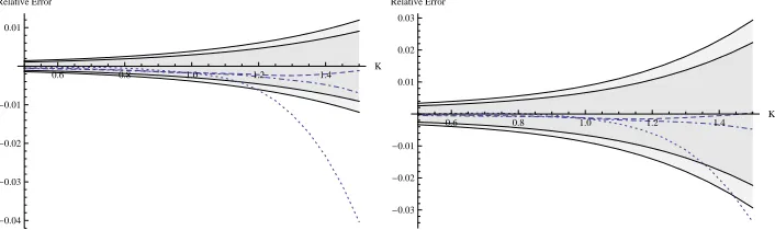
and fourth order approximation of the Call price with an accurate Monte Carlo (MC) simulation. In Figure 1 the dotted, dot-dashed and dashed lines represent the relative errors of the (second, third and fourth order, respectively) approximated Call prices, for maturities T = 0.25 (left) and
T = 1 (right). The values of the parameters are
K = 1, r= 5%, σ0= 20%, a= 1, (4.37)
and the initial priceS0 ranges from 0.5 to 1.5. A 200-steps Euler
0.6 0.8 1.0 1.2 1.4 K
-0.05 0.05 Relative Error
0.6 0.8 1.0 1.2 1.4 K
[image:16.595.121.477.125.233.2]-0.04 -0.03 -0.02 -0.01 0.01 Relative Error
Figure 1: Relative errors of the second (dotted line), third (dot-dashed line) and fourth (dashed line) order approximated Call prices (compared with MC prices). The 95% and 99% MC confidence regions are marked by gray and light gray re-spectively. A 200-steps Euler discretization of the SDEs and a MC with 1.000.000 simulations have been used. The parameters are as in (4.37) andT = 0.25 (left) andT = 1 (right)
0.6 0.8 1.0 1.2 1.4 K
-0.04 -0.03 -0.02 -0.01 0.01 Relative Error
0.6 0.8 1.0 1.2 1.4 K
-0.03 -0.02 -0.01 0.01 0.02 0.03 Relative Error
Figure 2: Relative errors of the second (dotted line), third (dot-dashed line) and fourth (dashed line) order approximated Call prices (compared with MC prices). The 95% and 99% MC confidence regions are marked by gray and light gray re-spectively. A 500-steps Euler discretization of the SDEs and a MC with 1.000.000 simulations have been used. The parameters are as in (4.37) andT = 2 (left) and
T = 3 (right)
other words, according to the MC approximation, the true price belongs to the gray (light gray) region with probability 95% (99%).
In Figure 2 we repeat the same experiment for longer maturities, T = 2 (left) and T = 3 (right): in this case a 500-steps Euler discretization has been used.
Next we consider the classical CEV model introduced by Cox [9]:
dSt=µStdt+σStβdWt. (4.38)
We are interested in this particular LV model because the difficulties in the numerical approximation of the CEV model are similar to those of the SABR model that is its stochastic volatility counterpart and is widely used to price interest rate options. These difficulties are mainly caused by the fact that if
[image:16.595.121.474.330.435.2]and Brecher [27]). As soon as S reaches zero, we have to keep it equal zero (absorbing boundary): under this condition, Delbaen and Shirakawa [11] proved the existence of a unique equivalent martingale measure under which the dynamics ofS are as in (4.38) with µ=r (r denotes the risk-free rate); moreover the arbitrage free price at time t, of the option which pays
ϕ(ST) at time T, is given by
C(t, S) =e−r(T−t)EhϕSTt,Si. (4.39)
Notice that, if we assume the origin as a reflecting boundary then the CEV model admits arbitrage opportunities (cf. [11] or [22]).
The density ofScan be expressed explicitly in terms of special functions: precisely, forr= 0 we have
Γ(t, S;T, y) =
√yS1 2−2βe−
S2(1−β)+y2(1−β)
2(1−β)2σ2(T−t)
(1−β)σ2(T−t) I2(1−1β)
(Sy)1−β (1−β)2σ2(T−t)
,
(4.40) whereIν(x) is the modified Bessel function of the first kind defined by
Iν(x) =
x
2
νX∞
k=0
x2k
22kk!G(ν+k+ 1)
and G is the Gamma function. For the caser 6= 0, we refer for instance to Davydov and Linetsky [10].
More explicit results on the precise asymptotic behaviour of Γ at bound-ary points have been recently proved by Ekstr¨om and Tysk [13]: in the case
r= 0 and β ∈[1/2,1[, they prove that
y7→Γ(t, S;T, y) ∼ y1−2β asy→0+.
Notice that, due to absorption, the law ofSTt,S has a Dirac delta component at the origin and consequently the function Γ in (4.40) is not a density in the standard sense because
Z +∞
0
Γ(t, S;T, y)dy <1,
-1 1 2 3
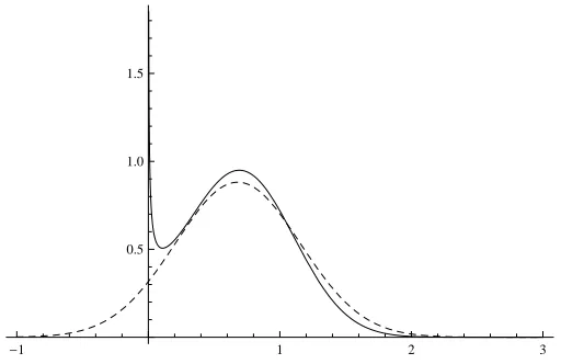
[image:18.595.169.425.125.291.2]0.5 1.0 1.5
Figure 3: CEV (solid line) and Gaussian (dashed line) densities
Remark 4.1. It is not restrictive to assume, as we shall systematically do in the sequel, that S0= 1: indeed, we can always rescale the CEV equation by setting Xt= SS0t and we get
dXt=rXtdt+σIXtβdWt
where σI =σS0β−1 is the so-called CEV normalized volatility. Even in the
case of interest rate models where S represents an interest rate with values of the order of1%, typically σI ranges from 10% to 50%.
The relationship between CEV stochastic equations and PDEs was es-tablished by Janson and Tysk [24] who proved a Feynman-Kac type theorem: precisely, they showed that, if the payoff functionϕis continuous and poly-nomially bounded (i.e. |ϕ(S)| ≤ C(1 +Sm) for some C and m), then the function C in (4.39) is the unique, polynomially bounded classical solution
to problem
LβC(t, S) = 0, (t, S)∈]0, T[×]0,+∞[,
C(T, S) =ϕ(S), S >0, C(t,0) =e−r(T−t)ϕ(0), t∈]0, T[,
(4.41)
where
Lβ =
σ2S2β
2 ∂SS+rS∂S+∂t+r, S >0.
Applying the 2nd-order approximation result of Section 2 directly to problem (4.41), we get exactly the classical Hagan-Woodward [19] formula for Call prices: notice that the true density ofST is supported onR+but it
satisfy the uniform parabolicity condition (3.29): thus, for moderately large values ofσ and for long maturities, we have a “loss of mass” of the Hagan-Woodward (HW) approximated density on R+ and consequently, as it has
been recognized by several authors, the HW approximation may become inaccurate.
To partially fix this problem, we suggest to first perform the change of variable S = ex to transform the Cauchy problem (4.41), posed on the semi-strip ]0, T[×R+, into problem
(
Lβu(t, x) = 0, (t, x)∈]0, T[×R,
u(T, s) =ϕ(ex), x∈R, (4.42)
with
Lβ =
σ2e2(β−1)x
2 (∂xx−∂x) +r∂x+∂t+r.
Since Lβ is defined on the entire real axis, it seems more natural to use of the heat kernel expansion to approximate its fundamental solution; once we have the approximation, we go back to the original variables to estimate the density ofS: we call this procedure the Log-approximation of the CEV density. The idea is that, while the HW approximation shifts part of the mass into the negative real axis, on the contrary the Log-approximation tries to mimic the delta at zero by concentrating part of the mass close to the origin. As we shall see later, the Log-approximation gives rather satisfactory results whenβ is not too close to zero, that is when the CEV model is not close to the normal one.
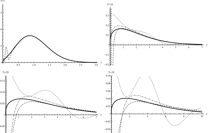
Figure 4 shows the graph of the CEV density
y 7→ Γ(0, S0;T, y)
in (4.40) withS0= 1,β= 23,σ= 0.5,r= 0 and maturitiesT = 1,10,20,30.
For comparison we also plot the approximation by Henry-Labord`ere (cf. [21], p.132), the HW approximation and the 4th-order Log-approximation of Γ. In Figure 5 we consider the caseβ = 13.
Notice that the LH, HW and Log approximations cannot reproduce the delta component of the CEV process at the origin and can take negative values. On the other hand, the integral over R+ of the Log-approximated
density is, by construction, equal to one (cf. Remark 2.5)
Z +∞
0
ΓLog(0, S0;T, y)dy = 1
for any positiveT andS0. This is not the case for the Gaussian
approxima-tion by Hagan-Woodward that verifies
Z +∞
0
0.5 1.0 1.5 2.0 2.5 3.0 y 0.2 0.4 0.6 0.8 T=1
1 2 3 4 5 6 7
y -0.2 -0.1 0.1 0.2 0.3 T=10
1 2 3 4 5 6 7
y -0.10 -0.05 0.05 0.10 0.15 0.20 T=20
2 4 6 8 10
[image:20.595.119.475.127.359.2]y -0.04 -0.02 0.02 0.04 0.06 0.08 T=30
Figure 4: CEV density with β = 2
3 (thick line), HL approximation (dot-dashed
line), HW approximation (dotted line) and 4th-order Log-approximation (dashed line) with parametersS0= 1,σ= 0.5,r= 0 and maturitiesT = 1,T = 10,T = 20
andT = 30
0.5 1.0 1.5 2.0 2.5 3.0
y 0.5
1.0 1.5 T=1
1 2 3 4 5 6 7
y -0.2 -0.1 0.1 0.2 0.3 T=10
1 2 3 4 5 6 7
y
-0.05 0.05 0.10 0.15 T=20
2 4 6 8 10 y
-0.04 -0.02 0.02 0.04 0.06 0.08 0.10 T=30
Figure 5: CEV density with β = 1
3 (thick line), HL approximation (dot-dashed
line), HW approximation (dotted line) and 4th-order Log-approximation (dashed line) with parametersS0= 1,σ= 0.5,r= 0 and maturitiesT = 1,T = 10,T = 20
[image:20.595.122.475.432.659.2]Integral of the HW approx.
0 10
20 30
Time
0.1
0.2
0.3
0.4
0.5
Volatility 0.4
0.6 0.8 1.0
Figure 6: Integral of the HW density as a function of the volatilityσ∈[5%,50%] and maturityT ∈[1
2,30] in the CEV model withβ = 1 2
In Figure 6 the value of the integral in (4.43), expressed as a function of the volatility σ ∈[5%,50%] and maturity T ∈[12,30], is plotted; the other parameters areβ = 12,r= 0 andS0 = 1. Also the integral of the LH density
is generally different from one, as shown in Figure 7.
Call and Put prices (×10)
Bessel 4th-Log 2nd-Log HW Call HW Put LH Call LH Put
T = 1 1.19345 1.19345 1.19344 1.19346 1.19174 1.19359 1.1939
T = 5 2.63769 2.63768 2.63737 2.63855 2.40181 2.64278 2.70363
T = 10 3.67286 3.67295 3.67201 3.67825 2.39639 3.69572 3.53664
T = 20 5.01275 5.01915 5.02073 5.0513 1.97434 5.11899 3.14135
T = 30 5.89194 5.91281 5.92962 6.00219 1.64068 6.14735 1.87179
Table 1: ATM Call and Put options in the CEV model withβ = 12,σ= 30% andr= 0 computed by convolution with the “Bessel” density in (4.40) (sec-ond column), the 4-th order Log-approximated density (third column), the 2-nd order Log-approximated density (fourth column), the Hagan-Woodward approximated density (fifth and sixth columns) and the Henry-Labord`ere approximated density (seventh and eighth columns)
This fact is noteworthy because when the integral in (4.43) is different from one, then option prices produced by the approximated density ΓHW
Integral of the LH approx.
0 10
20 30
Time
0.1
0.2
0.3
0.4
0.5
Volatility
-0.5
0.0 0.5
1.0
Figure 7: Integral of the LH density as a function of the volatility of the volatility
σ∈[5%,50%] and maturityT ∈[1
2,30] in the CEV model withβ= 1 2
σ = 30%, r = 0, K =S0 = 1, we report the numerical results obtained by
direct integration of the payoff functions of Call and Put options, convoluted with the “Bessel” density in (4.40) (second column), with the 4-th order Log-approximated density (third column), with the 2-nd order Log-Log-approximated density (fourth column), with the Hagan-Woodward approximated density (fifth and sixth columns) and with the Henry-Labord`ere approximated den-sity (seventh and eighth columns) respectively. In Table 2 we report the analogous results in the caseβ = 101 .
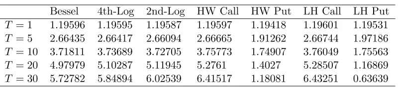
For the Bessel and Log-approximated densities, Puts and Calls have indeed the same price and in the table we report the common value; on the contrary, Put prices in the HW and LH approximations become uncorrect for long maturities and violate the Put-Call parity formula.
We recall that Hagan and Woodward give in [19] a well-known approx-imation formula of the implied volatility: the formula is rather satisfactory because it is obtained from the approximation of Call prices that are not affected by the singularity of the density at the origin. However, as the previous analysis shows, the HW approximation is less satisfactory from the more general point of view of the estimate of the density function, especially for pricing purposes.
Call and Put prices (×10)
Bessel 4th-Log 2nd-Log HW Call HW Put LH Call LH Put
T = 1 1.19596 1.19595 1.19587 1.19597 1.19418 1.19601 1.19531
T = 5 2.66435 2.66417 2.66094 2.66665 1.91262 2.66744 1.97186
T = 10 3.71811 3.73689 3.72705 3.75773 1.74907 3.76049 1.75563
T = 20 4.97979 5.10287 5.11945 5.2761 1.4027 5.28507 1.16869
[image:23.595.119.520.142.231.2]T = 30 5.72782 5.84894 6.02539 6.41517 1.18081 6.43251 0.63639
Table 2: ATM Call and Put options in the CEV model withβ = 101,σ= 30% andr= 0 computed by convolution with the “Bessel” density in (4.40) (sec-ond column), the 4-th order Log-approximated density (third column), the 2-nd order Log-approximated density (fourth column), the Hagan-Woodward approximated density (fifth and sixth columns) and the Henry-Labord`ere approximated density (seventh and eighth columns)
from 12 to 2, maturities from101 to 30 years and typical values of the volatility
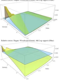
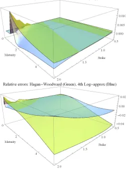
σ = 30% and σ = 80%. We first consider maturities T ≤ 5: in Figures 8 and 9 we plot the relative errors forβ = 23 and β = 13 respectively. Figures 10 and 9 are analogous but for longer maturities, up to 30 years.
References
[1] F. Antonelli and S. Scarlatti, Pricing options under stochastic volatility: a power series approach, Finance Stoch., 13 (2009), pp. 269– 303.
[2] J. P. Barjaktarevic and R. Rebonato,Approximate solutions for the SABR model: Improving on the Hagan expansion, Talk at ICBI Global Derivatives Trading and Risk Management Conference, (2010).
[3] E. Benhamou, E. Gobet, and M. Miri,Expansion formulas for Eu-ropean options in a local volatility model, Int. J. Theor. Appl. Finance, 13 (2010), pp. 603–634.
[4] H. Berestycki, J. Busca, and I. Florent,Computing the implied volatility in stochastic volatility models, Comm. Pure Appl. Math., 57 (2004), pp. 1352–1373.
Figure 8: Relative errors for Call prices in the HW approximation (green) and 4th Log-approximation (blue) forβ =2
3, maturitiesT ∈ 1
10,5
andσ= 30% (top) and
σ= 80% (bottom)
[6] W. Cheng, N. Costanzino, J. Liechty, A. Mazzucato, and V. Nistor,Closed-form asymptotics and numerical approximations of 1D parabolic equations with applications to option pricing, to appear in SIAM J. Fin. Math., (2011).
[7] R. Constantinescu, N. Costanzino, A. L. Mazzucato, and V. Nistor,Approximate solutions to second order parabolic equations. I: analytic estimates, J. Math. Phys., 51 (2010), pp. 103502, 26.
[8] F. Corielli, P. Foschi, and A. Pascucci,Parametrix approxima-tion of diffusion transiapproxima-tion densities, SIAM J. Financial Math., 1 (2010), pp. 833–867.
Figure 9: Relative errors for Call prices in the HW approximation (green) and 4th Log-approximation (blue) forβ =1
3, maturitiesT ∈ 1
10,5
andσ= 30% (top) and
σ= 80% (bottom)
[10] D. Davydov and V. Linetsky,Pricing and hedging path-dependent options under the CEV process, Management Science, 47 (2001), pp. 949–965.
[11] F. Delbaen and H. Shirakawa, A note on option pricing for the constant elasticity of variance model, Asia-Pacific Financial Markets, 9 (2002), pp. 85–99. 10.1023/A:1022269617674.
[12] P. Doust,No arbitrage SABR, working paper, (2010).
[13] E. Ekstr¨om and J. Tysk,Boundary behaviour of densities for non-negative diffusions, preprint, (2011).
Figure 10: Relative errors for Call prices in the HW approximation (green) and 3rd Log-approximation (blue) forβ = 2
3, maturitiesT ∈[5,30] andσ= 30% (top)
andσ= 80% (bottom)
[15] J.-P. Fouque, G. Papanicolaou, R. Sircar, and K. Solna, Sin-gular perturbations in option pricing, SIAM J. Appl. Math., 63 (2003), pp. 1648–1665 (electronic).
[16] J. Gatheral, E. P. Hsu, P. Laurence, C. Ouyang, and T.-H. Wang, Asymptotics of implied volatility in local volatility models, to appear in Math. Finance, (2010).
[17] P. Hagan, D. Kumar, A. Lesniewski, and D. Woodward, Man-aging smile risk, Wilmott, September (2002), pp. 84–108.
Figure 11: Relative errors for Call prices in the HW approximation (green) and 3rd Log-approximation (blue) forβ = 1
3, maturitiesT ∈[5,30] andσ= 30% (top)
andσ= 80% (bottom)
[19] P. Hagan and D. Woodward, Equivalent Black volatilities, Appl. Math. Finance, 6 (1999), pp. 147–159.
[20] P. Henry-Labord`ere, A general asymptotic implied volatility for stochastic volatility models, Frontiers in Quantitative Finance, Wiley, (2008).
[21] , Analysis, geometry, and modeling in finance, Chapman & Hall/CRC Financial Mathematics Series, CRC Press, Boca Raton, FL, 2009. Advanced methods in option pricing.
[23] S. Howison,Matched asymptotic expansions in financial engineering, J. Engrg. Math., 53 (2005), pp. 385–406.
[24] S. Janson and J. Tysk, Feynman-Kac formulas for Black-Scholes-type operators, Bull. London Math. Soc., 38 (2006), pp. 269–282.
[25] D. Kristensen and A. Mele,Adding and subtracting Black-Scholes: A new approach to approximating derivative prices in continuous time models, to appear in Journal of Financial Economics, (2011).
[26] A. Lesniewski,Swaption smiles via the WKB method, Mathematical Finance Seminar, Courant Institute of Mathematical Sciences, (2002).
[27] A. Lindsay and D. Brecher,Results on the CEV Process, Past and Present, SSRN eLibrary, (2010).
[28] A. Pascucci, PDE and martingale methods in option pricing, Boc-coni&Springer Series, Springer-Verlag, New York, 2011.
[29] L. Paulot, Asymptotic Implied Volatility at the Second Order with Application to the SABR Model, SSRN eLibrary, (2009).
[30] W. T. Shaw,Modelling financial derivatives with Mathematica, Cam-bridge University Press, CamCam-bridge, 1998. Mathematical models and benchmark algorithms, With 1 CD-ROM (Windows, Macintosh and UNIX).
[31] S. Taylor, Perturbation and symmetry techniques applied to fi-nance, Ph. D. thesis, Frankfurt School of Finance & Management. Bankakademie HfB, (2011).
[32] A. E. Whalley and P. Wilmott, An asymptotic analysis of an optimal hedging model for option pricing with transaction costs, Math. Finance, 7 (1997), pp. 307–324.
![Figure 10: Relative errors for Call prices in the HW approximation (green) andand3rd Log-approximation (blue) for β = 23, maturities T ∈ [5, 30] and σ = 30% (top) σ = 80% (bottom)](https://thumb-us.123doks.com/thumbv2/123dok_us/7846372.734919/26.595.172.424.136.475/figure-relative-errors-prices-approximation-andand-approximation-maturities.webp)
![Figure 11: Relative errors for Call prices in the HW approximation (green) andand3rd Log-approximation (blue) for β = 13, maturities T ∈ [5, 30] and σ = 30% (top) σ = 80% (bottom)](https://thumb-us.123doks.com/thumbv2/123dok_us/7846372.734919/27.595.173.424.137.475/figure-relative-errors-prices-approximation-andand-approximation-maturities.webp)
