The Distribution of an Index of Dissimilarity for Two Samples from a Uniform Population

(1)

The Distribution of an Index of Dissimilarity for

Two Samples from a Uniform Population

Giovanni Girone, Antonella Nannavecchia

Faculty of Economics, University of Bari, Bari, Italy Email: [email protected]

Received October 11, 2012; revised January 6, 2013; accepted January 19, 2013

Copyright © 2013 Giovanni Girone, Antonella Nannavecchia. This is an open access article distributed under the Creative Commons Attribution License, which permits unrestricted use, distribution, and reproduction in any medium, provided the original work is properly cited.

ABSTRACT

In this paper the authors study the sample behavior of the Gini’s index of dissimilarity in the case of two samples of equal size drawn from the same uniform population. The paper present the analytical results obtained for the exact distribution of the index of dissimilarity for sample sizes n≤ 8. This result was obtained by expressing the index of dissimilarity as a linear combination of spacings of the pooled sample. The obtained results allow to achieve the exact expressions of the moments for any sample size and, therefore, to highlight the main features of the sampling distributions of the index of dissimilarity. The present study can enhance inferential statistical aspects about one of the main contributions of Gini.

Keywords: Index of Dissimilarity; Uniform Distribution; Spacings

1. Introduction

In 1915 Corrado Gini [1] introduced, as an index of dissimilarity between two groups of observations, the mean of the differences in absolute value between co-ranked observations. Fifty years later, in 1965, Gini [2] pub- lished a comprehensive and systematic overview of his own and of other authors results about dissimilarity.

We assume that two groups have equal number of observations n. Let x x11, 12, , x1i, , x1n and 21 22 ,

2 2n

, ,

x x 

, ,

i

x  x

, ,

i

be the set of the observations in the first and in the second group respectively. Let _{1 1}_{ } _{1 2}_{ } ,

   

1 1n

, ,

x x 

x  x and x_{2 1}_{ },x_{2 2}_{ }, , x₂_{ }_i,,x₂_{ }_n be the observations arranged in non-descending order of magni- tude, respectively in the first and in the second group. Gini’s simple index of dissimilarity is given by

   

1 2

1 _.

n

i i

i

x x D

n 

 



If the two groups of observations are random samples, the distribution of the Gini index with samples drawn from the same population is of great interest for inferential purposes (e.g. to verify the homogeneity of two po- pulations).

As far as we know, the distribution of the index of dissimilarity between two samples has not been studied in

depth yet, maybe for the complex structure of the index which considers observations arranged in order of mag- nitude, co-ranked pairs and differences in absolute value. Instead the distribution of the index of dissimilarity between a sample and its population was obtained by For- cina and Galmacci [3] for the particular case of a discrete, equispaced and equidistributed population. The mean and variance of the distribution of the index of dissimilarity, both between two samples and between a sample and its population, have been obtained by Herzel [4] and Bertino [5] for some particular cases.

The purpose of this note is to study the sample behavior of the index of dissimilarity in the case of two samples from the same uniform population. In this paper we present the analytical results obtained for the exact distribution of the index of dissimilarity for sample sizes n≤

8 as well as for the exact general expressions of the main characteristic values (mean, variance, moments) of such a distribution for any sample size and their limiting values.

2. The Distribution of a Linear Combination

of Spacings

Let X X1, 2, , Xi, , Xn, be a random sample from a

(2)

 

1, 0 1, 0, elsewhere.

f x   x

 (1)

The variables of the sample in nondescending order

 1,  2, ,  i, ,  n

X X  X  X determine n1 spacings

         

     

1 2 1 1

1

0, ,

,1

, , _i _i ,

n n n

X X X X X

X X X



  

 

 

denoted by S S1, , , , ,2 Si  Sn1. These spacings are ex-

changeable random variables. Let

1 1 2 2 i i n1 n1,

Za S a S   a S   a S 

be their linear combination. Huffer and Lin [6] showed that the p.d.f. of Z_is

 

_

_









1 1

1 _,

1 ! i

i j

n r

p

i

r r

i i i _i _j j i

n y z h z

r y _y _y

 

 





 

  



  

  _ _ _

 

 





(2)

in which 1 2 p are the distinct values of

the weights ai with frequencies 1 2 p while

the sign +, appearing at the numerator of the ratio in the brackets, indicates that the function is nonzero only if it is positive. This result will be used for determining the p.d.f. of the index of dissimilarity.

, , , , ,_j

y y  y  y

, , , , ,_j

r r  r  r

3. The Index of Dissimilarity as a Linear

Combination of Spacings

The case of two independent random samples from uniform population with p.d.f. given by expression (1), both of size n, can be brought to the case of one random sample of size 2n from the same uniform population. Let

 1  2  i  2n be the 2n variables of the

pooled sample arranged in nondescending order of mag- nitude. They determine spacings

, , , , ,

X X  X  X

2n1

             

     

1 2 1 3 2 1

2 2 1 2

0, , , , , ,

,1 ,

j j

n n n

X X X X X X X

X X X



  

 

 

which we denote by S S1, , , , ,2  Sj  S2n1. Given all the





2 ,

   

2 ! ! !

h h

,k



n n  n n n subdivisions of the pooled sample into two samples of equal size n, let 1 2

and 1 2 i n be the ranks in the pooled sample

of the variables in the first and in the second sample respectively. Moreover

, , , , , hi hn

, , , ,

k k  k 



Min ,

i i i

p  h k

1, 2, ,

i  n

and

, for . It is easy to verify that the index of dissimilarity is given by





Max ,

i i i

q  h k

   





1 i i _,

n

q p

i

X X

D

n









or, when the differences are expressed in terms of spac-

ings

    1

,

i

i i

i

q h

q p

h p

X X S

 

 



by

1 1

, i

i

q n

h i h p

S D

n

  



 

clearly D is equal to the linear combination of spacings given by

1

,

n

h h h

D  a S





in which ah is the relative frequency of the n intervals i

1

i

p  q that contain the hth spacing. The above pro- cedure for each of the



2 ,n n



subdivisions of the pooled sample should be used to determine the p.d.f. of the index of dissimilarity. To reduce the amount of computation it is appropriate to aggregate the subdivisions which bring to the same coefficients ah. Due to the ex-

changeability of thespacings it is also appropriate to aggregate all subdivisions which bring to the same set of- frequencies. In practice the



2 ,



, , ,

y y

n n subdivisions are aggregated into groups characterized by the same set of frequencies. Denoting by 1 2 the distinct values of coefficients ah and by 1 2

their frequencies (see Paragraph 2) we can apply formula (2) with the only variant of replacing n with 2n. Taken together the subdivisions which have the same values

, ,

j

y y

 

, ,

r r p , , ,r_j  r_p



y r_j, _j



it is possible to proceed in an aggregate way by applying formula (2) only to homogeneous groups of subdivisions. These are in number of which allows to reduce considerably the amount of computation. Ob- viously, regard should be given to frequencies of the homogeneous subdivisions.

1 n

2

4. The Distributions of the Index of

Dissimilarity for Sample Size Up to 8

To generate the sampling distribution of the index of dissimilarity two programs have been developed for Mathe- matica software. The first one generates, for each value of n, the subdivisions of the first 2n natural numbers into two subsets of size n and proceeds to identify homogeneous typologies and to define their frequencies. The second one starts, for each value of n, with such typologies and frequencies and gives, by applying formula (2), the p.d.f. of the index of dissimilarity. It should be said that heaviness of both calculation and resulting expressions led us to stop at n8. The sampling densities of the index of dissimilarity (see Paragraph 2) are splines of order 2n− 1with knots at points i/n for

They are also unimodal between 0 and 1, extreme values

1, 2, , 1.

(3)

in which they assume value 0. The only exception is the degenerate case n1.

 

0,

f d



 









2

3

16 1

6 21 19 , for 0 ,

3 2

16 ₁ _for 1 _1,

3 2

0, elsewh . ,

ere

f d d d d d

d d

    

   



For n1





2 1 ,for 0 1, elsewhere.

d d

   

For n3 For n2

 













2 2 3

324 1

75 195 174 ,for 0 ,

5 3

243 1 2

for ,

20 3 3

243

1 for 1,

20 3

0, els

2

f d d d d d

d d

   

 

  

5

10

1 ,

ewh ,

. ere

d

 

For n4

 









3 2 3 4

2 3 4 5 6 7

2 3 4 5

8192 1890

196

2 171

 

24570 124362 287931 255625 ₁

, for 0 ,

945 4

8 843 35 307440 1283520 3037440 4193280 3161088 1008640 ₁ ₁

,for ,

945 4 2

8 885 109 36 73920 134400 129024 64512

d d d d d

f d d

d d d d d d d

d

d d d d d

   

  

      

  

   













6 ₁₃₃₁₂ 7

1 3

, for ,

945 2 4

8192 3

or 1,

315 4

0, elsewher

d d

d

d d



 

   



7

1 ,f

e. For n5

 







4 2 3 4

2 3 4 5

6 7

15625 1161216 23224320 192326400 818424000 1779880500 1576012625 , 36288

1 for 0 ,

5

25 184789 5314725 54573300 302410500 1031073750 2258943750 108864

3167062500 2702812500 123539

d d d d d

f d

d

d d d d d

d d

   



 

   

 



 

 



5 d





8 9

2 3 4 3

5 6 7 8 9

0625 212656250 ₁ ₂

, for ,

108864 5 5

25 208427 2703195 17311500 68533500 178526250 68533500 178526250 108864

311456250 360937500 267187500 114609375 21718750 ₂ ₃

for ,

108864 5 5

2 77

,

5 2

d d

d

d d d d d

d



 

    

 

  

 





4 d







2 3 4 5

7 8 8 9

9

69 839745 6308100 23320500 51108750 71268750 64312500 108864

36562500 11953125 11953125 1718750 ₃ ₄

for ,

108864 5 5

1953125 1 _{, for} 4 _1,

36288 5

0, elsewh

,

ere.

d d d d d d

d d d d

d t

d

    

 

 



  



 

6



(4)

For n6

 







5 2 3

4 5 6

2 3 3

69984 2464000 70224000 860640000 5771535000 9625

22234481500 46488497110 41096463787 ₁

+ ,for 0 ,

9625 6

39390245 596300430 56212110900 985055920200 985055920200 8951408690400 277200

d d d d

f d

d d d

d

d d d d

  



 

 

     



4 d



5 6 7 8

9 10 11

2

0

51025364026560 195684595666560 516532350470400 930778647955200 2772000

1098045852710400 766505627458560 240526446437376 ₁ ₂

,for ,

2772000 6 6

268638245 8109363570 98322929100 6828960

d d d d

d d d

d

t t

 



 

   

 









3 4

5 6 7 8

9 10 11

79800 3088638669600 2772000

9630608581440 21202538797440 33029606649600 35735384044800 2772000

25604654169600 10945788733440 2116759578624 ₃

,for ,

2772000 6 6

15235805 275015730 2

4

01

t t

t t t t

t t t

d d



 

  



 

  













2 3 4

5 6 7 8

9 10 11

11

9609900 8379142200 22327034400 308000

40613348160 51839948160 46651334400 29099347200 308000

12009254400 2956124160 329204736 ₄ ₅

,for ,

308000 6 6

209952 1 _{, for} 5 _1,

1925 6

0, elsewhe

d d d

d d d d

d d d

d t

d



 



  

 

 











re. For n7

 





6 2

3 4

6 7

5764801 12809871360000 493180047360000 8375654327040000 100077120000

80940502843200000 478835085704976000 1728741146238943200 100077120000

3517908542952383580 3106403114212520549 1000771

d d

f d

d d

 



 



 

5 d

d



2 3

4 5

7

1 ,for 0 ,

20000 7

49 705190243035 48608926614885 1370336931078570 21075409844719230 400308480000

205665941648192025 1375788745611094815 6560947022693803740 400308480000

22672129451401209780 5

d

d d

d

 

  



 



 

6 d

d



8 9

10 11

12 13

6718764070636913245 100876943897061006675 400308480000

122406144806654198490 93386013407104353390 400308480000

37532683619581030335 4652108914707165149 ₁ ₂

,for ,

400308480000 7 7

d d

d

 





(5)



2 3

4 5

7 8

49 724389014235 26416076080485 495975655072170 5590840507682430 400308480000

41412935739200025 213611632848829215 794177103242462940 400308480000

2166089514477868980 4351951762561047645 6

d d

  



 



 



6 d

d



9

10 11

12 13

381666843892014675 400308480000

6655537983365961690 4684154434862346990 400308480000

1997194022429995935 390116369319886349 ₂ ₃

, for ,

400308480000 7 7

49 386280677245 7878437015995 7787217313

d

d d

 



 

 







2 3

4 5 6

7 8

10

2390 478219347415810 133436160000

2005934860104175 6039667172443905 13424962922350980 133436160000

22336958123139660 27870188207576715 25798612790675725 133436160000

17243777843522230

d d

d d d

d



 



 



 

9





11

12 13

2 3

4

7888169349117330 133436160000

2214635612061145 288256669921283 ₃ ₄

, for ,

133436160000 7 7

49 218508517245 4061620375995 37795598412390 221061326295810 133436160000

880868517704175 2495708193

d

d d

d

d d

d



 

  



 

d





5 6

7 8 9

10 11

12 13

883905 5155725305710980 133436160000

7865792294019660 8876783056856715 7332802227475725 133436160000

4317710449282230 1718909910957330 133436160000

415268275931145 46034143903783 133

d d

d d d

d d



 



 



2 3

4 5 6

7 8

4 5

, for ,

436160000 7 7

49 22582874919 406770055419 3232969102818 15243712005522 6671808000

47995298235885 107152175090961 175163892980076 6671808000

212840606870892 192597579807633 1283662

d

d d d

d d

 

   



 

 







9

10 11

12 13

13

36243245 6671808000

61318032201426 19895861688066 6671808000

3932902891827 357896140483 ₅ ₆

, for ,

6671808000 7 7

96889010407 1 6 , for 1,

444787200 7

0, elsewhere.

d

d d

d t

d

 



  



  

(6)

For n8

 

7



2

3 4 5

6 7

34359738368 5028288890625 251414444531250 5647327122937500 5028288890625

74128599182137500 619867652797575000 3372166777264740000 5028288890625

11629230369678054000 23201017571436730200

d d d

f d

d d d

d d

 

 

 

 





8

2

3 4

20470385435095442888 ₁ , for 0 ,

5028288890625 8

1785866560504985 98858130907162200 1620233588120347200 20113155562500

10557759586230438400 787748798010873753600 14297410591221007810560 20113155

d

d d

d d d



 

 



 



5

6 7

8 9

10

562500

154167083013468081356800 1145320397304538123468800 20113155562500

6195682772044929721958400 24964730331199205644697600 20113155562500

75264504448998097110958080 16803488492353234686443

d d

d





 

 



11

12 13

14 15

5200 20113155562500

270307440945096620716851200 296825455668996496529817600 20113155562500

199459902900530267868364800 61946662652365112780783616 ₁ ₂

, for ,

20113155562500 8 8

10395733767175

d

d d

d



  



 





2

3 4

6 7

015 472434555633637800 9801917876430052800 20113155562500

125944461384016038400 1123561463695660953600 7357990590660920770560 20113155562500

36458070001964567756800 138927791089112894668800

d d

 

 



 

5 d

8 9

10 11

12

20113155562500

410010935467157382758400 936551720499415718297600 20113155562500

1641822440995120301998080 2169256345186226877235200 20113155562500

2091386543607603475251200 138933858872327

d d

d td

d

 





13

14 15

2

9403417600 20113155562500

568841319984036367564800 108244770034492549103616 ₂ ₃

, for ,

20113155562500 8 8

12094942095795265 419329681293847800 6550593682374772800 20113155562500

622576647567731

d

d d

d

d d



 

  

 



3 4

6 7

58400 405139576487996313600 1917540769129588162560 20113155562500

6830701536285904076800 18670785557317602508800 20113155562500

d d d

d d

 

 

(7)

8 9

10 11

12 13

39519036698073130598400 64821603114625374617600

20113155562500

81770292390085609390080 77939848950584652595200

20113155562500

54354818157071512371200 26190616878873418137600

201131555625

d d

 





14 15

2

3 4

00

7798288061683256524800 1081819211351107567616 ₃ ₄

, for ,

20113155562500 8 8

476110953668245 8404005584717400 72266127037742400

6704385187500

368690549064947200 1106957686081228800 136951527

d d

d

d d



 

 



 





5

6 7

9 10

0856212480 6704385187500

3486454449904025600 22178074859510169600 59187514072419532800

6704385187500

101932925346591539200 123260133914821263360 106598507655620198400

6704385187500 650190

d

d d







  



8

11

d





12 13

14 15

2

72070706790400 26694919115715379200

6704385187500

6643496645138841600 759154504863055872 ₄ ₅

, for ,

6704385187500 8 8

138678600249637 3026020675659240 31705558016274240

670438518750 206589742

d d

d

d d



 

 







3 4

6 7

8 9

406494720 925355068608122880 3004552263085621248

670438518750

7298289851009597440 13513030837248983040

670438518750

19250589909878046720 21128554437756846080

670438518750 177429597020372336

d d d

d d

 

 



5



10 11

12 13

14 15

64 11208493302452060160

670438518750

5161209629203496960 1636889689514311680

670438518750

319966130020024320 29078234263977984 ₅ ₆

, for ,

670438518750 8 8

12192935458067 233760762334680

d d



 



 

  







2

3 4 5

6 7 8

9

2043259180052160 26817540750

10869414530024960 39517814160814080 104311825731649536

26817540750

206943775415336960 314693685576990720 370262962360811520

26817540750

337377216755138560 236

d

d d d

d

 



 

  

10 11

297127330840576 125003004515450880

26817540750

d  d

(8)







12 13

14 15

15

48370608882319360 12930256742645760 26817540750

2135801336954880 164376988352512 ₆ ₇

, for ,

26817540750 8 8

274877906944 1 7 , for 1.

638512875 8

d d

d t

d

 



 



  



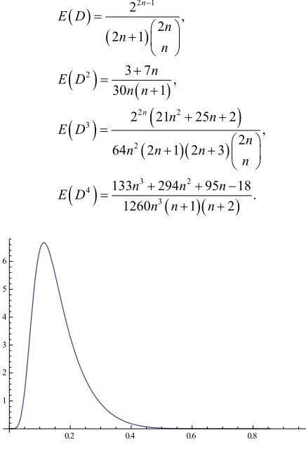
The sampling distribution of the index of dissimilarity for n7 is shown in Figure 1.

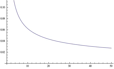
Based on these moments, we could study the main features of the sampling distribution of the index of dissimilarity starting from the mean. The trend of the mean with increasing sample size is shown in Figure 2.

5. The Moments of the Sampling

Distribution of the Index of Dissimilarity

It can be seen, the mean decreases for increasing n and it goes to zero for . The trend of the mean multiplied by

n 

n is increasing and converges to π 4 (Figure 3).

On thee basis of the sampling distributions of the index of dissimilarity (see Paragraph 4), we obtained the values ofthe mean and of the second, third and fourth moment

about the origin reported in Table 1. _{of dissimilarity can be expressed as follows}The variance of the sampling distribution of the index

Using the moments of the Dirichelet distribution, which is the model of the joint distribution of uniform spacings, as well as the expressions of the moments of a linear combination of equally distributed random variables, we obtained the mean and the second, third and fourth moment of the sampling distribution of the index of dissimilarity:



_{ }

_

2

2 1

2 3 7 2

2 .

30 1

2 1

n

D

n

n n n

n n

 

 

 

 _ _

 

 

  



  

  

 

The trend of the standard deviation with increasing sample size is shown in Figure 4.

 





 

_

_

 











 

_

_

_

2 1

2

2 2

3

2

3 2

4

3

2 _,

2 2 1

3 7 _,

30 1

2 21 25 2

, 2 64 2 1 2 3

133 294 95 18 .

1260 1 2

n

E D

n n

n n E D

n n

n n

E D

n

n n n

n

n n n

E D

n n n 



 

  

 

 



 



 

 _{  }

 

  



 

It can be seen that the standard deviation decreases with increasing n and it goes to zero for . The trend of the standard deviation multiplied by

n 

n is also

able 1. Mean and moments of the sampling distribution of T

the index of dissimilarity for sample size up to 8.

Moments about the origin Sample

Mean Fourth

size _{Second Third}

1

0.2 0.4 0.6 0.8 1.0

1 2 3 4 5 6

Figure 1. Sampling distribution of the index of dissimilarity

1

3

1 6

1 10

1 15 4

15

17 180

17 420

67 3360 2

3 8

35

1 15

19 810

271 28350

4 64

315

31 600

73 4620

2263 403200

5 128

693

19 450

2608 225225

1018 275625

6 512

3003

1 28

3632 405405

1661 635040

7 1024

6435

13 420

4288 595595

632 324135

8 16384

109395

59 2160

12368 2078505

[image:8.595.104.382.86.179.2] [image:8.595.352.495.317.378.2] [image:8.595.57.275.396.716.2] [image:8.595.309.537.482.732.2]

(9)

10 20 30 40 50 0.10

[image:9.595.53.286.65.569.2]

0.15 0.20

Figure 2. Trend of the mean with increasing sample size.

10 20 30 40 50

[image:9.595.58.285.78.226.2]

0.25 0.30 0.35 0.40

Figure 3. Trend of the mean multiplied by n with in- creasing sample size.

10 20 30 40 50

[image:9.595.312.535.85.226.2]

0.02 0.04 0.06 0.08 0.10

Figure 4. Trend of the standard deviation with increasing sample size.

decreasing and converges to 7 30π16 (Figure 5).

By converting moments about the origin into central ain indices of

ex

sample sizes up to the limit given by

moments it is possible to obt skewness and cess of kurtosis of the sampling distribution of the index of dissimilarity for a uniform population. Their trends with increasing sample size are shown in Figures 6 and 7.

It can be seen that distributions of the dissimilarity index are positively skewed and the skewness increases for increasing

10 20 30 40 50

0.192 0.194 0.196

Figure 5. Trend of the standard deviation multiplied by n with increasing sample size.

10 20 30 40 50

[image:9.595.309.537.266.411.2]

0.2 0.4 0.6 0.8 1.0 1.2

Figure 6. Trend of the skewness index with increasing sam- ple size.

10 20 30 40 50

0.5 1.0 1.5 2.0

Figure 7. Trend of the excess of kurtosis index with in- creasing sample size.









3 2 1.297.

4 56 15 π 

It is also clear that such distributions a e leptokurtic and this leptokurtosis increases for incre sing sample sizes up to the limit given by

3 15π 119 40 π

r a









2

3328 45 119 30π π

2.174.

56 15π

  



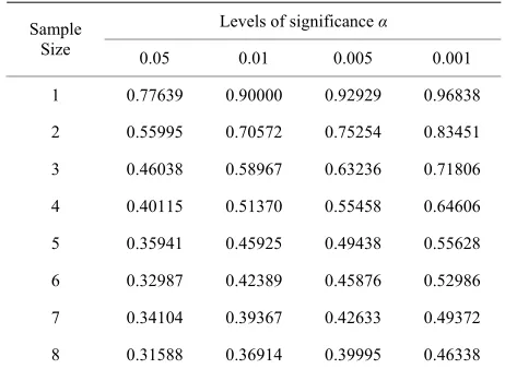
[image:9.595.58.286.434.572.2] [image:9.595.309.538.442.582.2]

(10)

[image:10.595.56.287.111.280.2]

Table 2. Thresholds of the sampling distribution of the in- dex of dissimilarity for sample size up to 8.

Levels of significance α Sample

Size _{0.05 0.01 0.005 0.001}

1 0.77639 0.90000 0.92929 0.96838

2 0.55995 0.70572 0.75254 0.83451

3 0.46038 0.58967 0.63236 0.71806

4 0.40115 0.51370 0.55458 0.64606

5 0.35941 0.45925 0.49438 0.55628

6 0.32987 0.42389 0.45876 0.52986

7 0.34104 0.39367 0.42633 0.49372

8 0.31588 0.36914 0.39995 0.46338

6. Thresholds of the Sampling Distributions

of

th

e In

dex of

Di

ssimila ty

ri

Thresholds at usual levels 0.05,0.01, 0.005, 0.001

are required to test statistical hypothesis that two samples me from the same uniform populat

co ion. Thresholds

act sampling distributions have been calculated on the ex

of the index of dissimilarity (see Paragraph 4) and their values are reported in Table 2. For larger sample sizes

can be used the approximate conservative thresholds

0.05 0.100 ,

0.01 0.116 ,

n n

 

 

0.001 0.126 ,

0.005 0.147 .

n n

 

 

7. Conclusions

In this note we obtained the distributions of the index of case of two random samples of sm

population. This result was obt dissimilarity in the

size from a uniform

all

ained [6] W. F. Huffer and C. T. Lin, “Spacings, Linear Combina- _{tions of,” In:}_{Encyclopedia of Statistical Sciences}_{, John}

Wiley & Sons Inc., New York, 2006, pp. 7866-7875.

by expressing the index of dissimilarity as a linear combination of spacings of the pooled sample. The exact

expressions, in the form of splines of order 2n− 1, were obtained for samples of size ≤ 8. Although it would be possible to go further we stopped at this size because of the heaviness in processing and in the resulting expressions. This limit could be overcome by using some al- ready set calculus programs. The obtained results allow to achieve the exact expressions of the moments and, therefore, to highlight the main features of the sampling distributions of the index of dissimilarity.

Beyond the problem of dealing with larger sample sizes, open problems are also those considering the case of two samples with different sizes as well as the case of other distribution models for population.

We believe that the present work has re-opened a re- search strand able to enhance also the inferential statistical aspects about one of the fundamental contributions of Gini.

REFERENCES

[1] C. Gini, “Di Una Misura Della Dissomiglianza tra Due Gruppi di Quantità e Delle Sue Applicazioni Allo Studio Delle Relazioni Statistiche,” Proceedings of the R. Vene-

tian Institute of Sciences, Literatures and Arts, Vol. 74,

1914, pp. 185-213.

[2] C. Gini, “La Dissomiglianza,” Metron, Vol. 24, No. 1-4, 1965, pp. 85-215.

[3] A. Forcina and G. Galmacci, “Sulla Distribuzione Dell’ Indice Semplice di Dissomiglianza,” Metron, Vol. 32, No. 1-4, 1974, pp. 361-378.

[4] A. Herzel, “Il Valor Medio e la Varianza Dell’Indice Semplice di Dissomiglianza Negli Universi dei Campioni Bernoulliano ed Esaustivo,” Library of Metron, Series C,

Notes and Reports, Vol. 2, 1963, pp. 199-224.

[5] S. Bertino, “Sulla Media e la Varianza Dell’Indice Sem- plice di Dissomiglianza Nel Caso di Campioni Proven- ienti da una Stessa Variabile Casuale Assolutamente Con- tinua,” Metron, Vol. 30, No. 1-4, 1972, pp. 256-281.