Efficient Heuristics for Flow Shop Scheduling with make span Optimization Criteria

(1)

(2)

Technology (IJRASET)

©IJRASET: All Rights are Reserved

541

Efficient Heuristics for Flow Shop Scheduling with

make span Optimization Criteria

Sunil Kumar1, Sanjay Jain2

Samrat Ashok Technological Institute, Vidisha, 464001, M.P., India)

Abstract: - In modern manufacturing environment the trend is the development of Computer Integrated Manufacturing (CIM) technologies which is computerized integration of manufacturing activities (design, planning, sequencing, scheduling and control).In the Flexible Manufacturing System (FMS), the productivity of CIM is highly depending upon the scheduling. FMS scheduling is a procedure to select the right future operational program of different operations, by sequencing through different work stations, operations, jobs, and routings with the efficient combination of the high flexibility of job shop type with high productivity of flow shop type. The flow shop scheduling problem is one of the well-known scheduling problems. In a flow shop environment scheduling of n jobs on m machines find prominent place in the field of production scheduling. The present work is focus on scheduling the jobs in a flow shop environment with make span minimization criteria in comparative fashion. In the proposed work there are three previous proposed heuristics Palmer’s, CDS and NEH have been analyzed and tested for the problem of 4 jobs with 4 machines consist processing time as input parameter. The objective of this thesis is to analyze various factors of each proposed scheduling methods for real world situation by the simulation using ProModel software. From the comparative analysis and use of simulation approach, the optimal make span and actual shop floor condition of each considered heuristic rules are described for each proposed problem and Graph charts, tables and simulation results were generated to verify the efficient utilization and effectiveness of FMS system.

Key words: Scheduling, FMS,Flow Shop Scheduling, Heuristic, Make Span.

I. INTRODUCTION

A. Sequencing and Scheduling

Scheduling is defined as an important tool in the manufacturing area since productivity is inherently linked to how well the resource is used to increase efficiency and reduce waste [1,2]. Scheduling is an essential operational task required in any large or small manufacturing network in order to allocate resources like robots and AGVs, to various competing entities such as job processing on the machines or workstation utilization. The main challenge is designing, selecting and adopting a good scheduling rule is in achieving a balance between performances and implimentability [3]. Flexible manufacturing system scheduling is concerned with the right allocation of machines to operation over time. It is an activity to selected the right future operation of jobs on the system of an optimal make span for allocating competitive different demands of different products delivery dates, and sequencing through different machines, operations and routings of jobs that’s for individual or combination the high flexibility of job shop type with high productivity of flow shop type scheduling criteria [4]

B. Relation between Flow Shop Scheduling and FMS

(3)

Technology (IJRASET)

542

scheduling plays an important role in most manufacturing and service system with same sequencing of jobs on all machines [5]. The flow shop contains m different machines on which n jobs are considered. Each of n jobs requires k operation and each operation are performed on a separate machine and k always be

k



m

. The flow of work is unidirectional; thus every job has been processed on same sequence. In other words, if machine i are numbered from 1.2,3,...m. then operations of job j will correspondingly be numbered (1,j), (2,j),(3,j),…(k,j). In this situation, each job has been assigned exactly m operations. But in real context a job may have fewer operations. Nevertheless, such a job will still be treated as processing m operations but zero processing time correspondingly. The general n jobs, m machines flow shop scheduling problem is quite formidable. Considering an arbitrary sequence of jobs on each machine, there are (n!)mpossible scheduleswhich poses computational difficulties. It is not always essential to consider (n!)m schedules in search for an optimal so that to make easy flow shop scheduling some heuristic approaches were developed by various researchers. After conclusion of various researchers that the affected heuristic reduced much of the deviation and computational difficulty linked with whole rescheduling and right shifting [6].

C. Heuristics

Heuristics technique is a specific schedule repair method, which does not guarantee to find an optimal schedule, but consists the capability to find reasonably better solution in a short duration. Widely existing schedule repairing heuristics are: match-up schedule repaired, right-shift schedule repair and partial schedule repair. The affected heuristic reduced much of the deviation and computational complexity associated with complete rescheduling and right shifting according to the conclusion of various researches.

Meta- heuristics are known as a high level heuristics which guide local search heuristics to ignore from local optima. In recent years meta-heuristics (tabu search, simulation annealing and fuzzy logic) have been efficiently used to resolve production scheduling tasks. Based on the idea of searching neighborhoods, local search heuristics are neighborhood search methods.In local neighborhood search, the search starts from some given solution and tries iteratively to get a well neighborhood in a mannered defined neighborhood of the instant solution using move operators. When no better solution can be found in the neighborhoods of the current solution which is the local optimum, then search process stops [15].

Since the flexible flow shop scheduling problem is Non- deterministic polynomial time hard (NP-hard), algorithms for finding an optimal solution in polynomial time are therefore unlikely to exist. Thus, heuristic methods are studied to find approximate solutions. Most researchers develop existing heuristics for the classical flexible flow shop problem with identical machines by using a particular sequencing rule for the first stage.

There are a various objectives to be reduced for flow shop scheduling some of them are total make span, mean lateness, tardiness, mean flow time based objectives etc. in the proposed work, for effective utilization of all the resources flow shop scheduling with make span criteria has been considered. Make span is the time length from the starting of the first operation of the first demand to the finishing of the last operation of the last demand. The three heuristics available in methodology viz. Palmer, CDS and NEH have been used and considered for the solution of the flow shop scheduling problem of 4 jobs and 4 machines in comparative manner. The classical flow shop scheduling problem is one of the most well-known scheduling problems. Now the problem is found as follows: There are 4 sets of jobs and a set of 4 machines. Each job contains series of operation; each of them needs to be processed during an uninterrupted time period of a given processing time on a given machine. Every machine can process maximum single operation at one time. A schedule is allocation of operations to time intervals of the machines. The problem is to find the schedule of minimum time length. The presented work tends to reduce the make span of batch-processing machines in a flow shop. The processing times and the sizes of the jobs are well known and different. The machines can process a batch as long as its capacity is not exceeded which is pre-defined. Consequently, comparison based on Palmer’s, Campbell, Dudek and Smith (CDS), Nawaz, Enscore, and Ham (NEH) heuristics are proposed. Gantt chart was generated to verify the effectiveness of the proposed approaches.

II. PROBLEM DESCRIPTION

(4)

Technology (IJRASET)

543

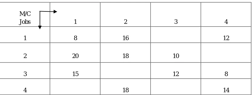
assumed to be ready which ever and whatever job is processed. Machine may be idle and pre- emption is not allowed. All four job sets are presented in next methodology chapter with processing time data was used by K.V.Subbaiah, 2009, in scheduling of AGVs and machines in FMS with make span criteria using sheep flock heredity algorithm [16].The problem data are given as jobsets.

M/C

Jobs 1 2 3 4

1 8 16 12

2 20 18 10

3 15 12 8

4 18 14

Table2: Processing time in Job set 1 Table2: Processing time in Job set 2

Table3: Processing time in Job set 3 Table 4: Processing time in Jobset 4

If the machines are numbered from 1, 2, 3…, m, then operations (k) of job (j) will correspondingly be numbered (1j, 2j, 3j…mj). In real situation context, each job may be assigned operation, less or equal to m, such a job will still be treated as processing m operations but with zero processing time correspondingly for the analytical solution.

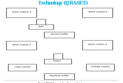
A. Flexible Manufacturing System Configuration

In the previous section, various parameters of system configuration have been identified. With the above parameter in mind, a conceptual FMS configuration as shown in figure 3.1 has been formulated. In present work the considered system configuration consists of 4 CNC workstations (M1, M2, M3, M4) and one robot and AGVs for the material handling. The system has to produce four type products (J1, J2, J3, J4).Each jobs required four or less than four different operations in real context

M/C

Jobs 1 2 3 4 1 9 11 7 2 19 20 13 3 14 20 9 4 11 16 8

M/C

Jobs 1 2 3 4 1 11 16 19 13 2 21 16 14 3 14 10 8 9 4 21 19 11 15 M/C

Jobs 1 2 3 4 1 12 9 9 2 11 16 9

(5)

Technology (IJRASET)

[image:5.612.101.504.58.331.2]

544

Fig. 1:FMS Layout for Current System

B. Assumptions

The following assumptions of considered problem for the existing FMS system are considered:

1) If jobs (j=1,2…n), machines (i=1,2,..m) and operations(k) always k≤m.

2) _{Each job set contains 4 different jobs and 4 different machines.} 3) _{Processing time need not be the same for all operations or jobs.} 4) _{Sequencing of machine will be same for all jobs.}

5) _{Every machine cannot processes more than one job at a time.} 6) _{Every job cannot processes on more than one machine at a time.} 7) _{Pre-emption is not allowed.}

8) _{The first machine is assumed to be ready which ever and whatever job is to processed.} 9) _{Machine may be idle.}

III. OBJECTIVES OF THESIS

A. To deal with the production planning problem of a flexible manufacturing system. We model the problem of a flow shop scheduling with the objective of minimizing the make span.

B. To provide a schedule for each job and each machine. Schedule provides the order in which jobs are to be done and it projects start time of each job at each work center.

C. To select appropriate heuristic approach for the scheduling problem through a comparative study.

D. To solve FMS scheduling problem in a flow-shop environment considering the comparison based on palmer’s heuristic, CDS heuristic and NEH heuristic rule. Graphs and table was generated to verify the effectiveness of the proposed approaches.

E. To select an efficient heuristic rule for the considered type of problem on the basis of actual shop floor condition by using simulation approach.

F. The objective of scheduling can yield: Efficient utilization of

1) Work stations

2) Resources

3) Facilities Minimization of

(6)

Technology (IJRASET)

545

2) Blockage

3) Avg. time in system

IV. METHODOLOGY

Fig.2: Block diagram of methodology

A. Heuristic Rules for Considered Problem 1) Heuristic rules for job set 1

a) Palmer’s heuristic rule for job set 1

This heuristic rule of scheduling comprise of three step as follow

Step 1: for n job and m machine problem of flow shop scheduling, compute slope index for job as follow

RESULTS

ES

Palmer’s Heuristic Method

(4jobs 4 Machines)

CDS Heuristic Method

(4jobs 4 machines)

NEH Heuristic Method

(4jobs 4 Machines)

Optimum make span on the basis of job sequencing

Simulation by ProModel Software Simulation by ProModel software Simulation by ProModel software

Average time in the system Average time in the operation

Blockage in the system Workstations utilization Flow shop scheduling

Problem Statement

Minimization of Make span

(7)

Technology (IJRASET)

546

=− −(2 −1)

Or

= ( −1) . + ( −3) . + ( −5) . +⋯ ⋯ −( −3) . −( −1) .

Step 2: make the sequence of the jobs based on the decreasing order of the slop index S j values as

≥ ≥ ≥ ⋯ ⋯

Step3:find out optimal sequence based as Sjtherefore compute the make span from original problem

Let us consider the job set 1 for solving by palmer’s heuristic rule

M/C

Jobs 1 2 3 4

1 8 16 12

2 20 18 10

3 15 12 8

[image:7.612.99.515.228.386.2]

4 18 14

Table 5: Processing time for job set 1 Solution is constructed as follows:

Step 1: slope index are computed on the basic of equation

=∑ { −(2 −1)} = =∑ {4−(2 −1)}

For the 4 job and 4 machine problems the above equation can be expanded as

= ( −1) + ( −3) −( −3) −( −1)

The slop index Sj for the Jth job as:

S1= {(4-1) x12} + {(4-3) x0}-{(4-3) x16}-{(4-1) x8}

= 36-40= -4

S2= {(4-1) x0} + {(4-3) x10}-{(4-3) x18}-{(4-1) x20}

= 10-78= -68

S3= {(4-1) x8} + {(4-3) x12}-{(4-3) x0}-{(4-1) x15}

= 36-45= -9

S4= {(4-1) x14} + {(4-3) x0}-{(4-3) x18}-{(4-1) x0}

= 42-18= 24

Step2: jobs are sequenced according:

≥ ≥ ≥

24≥ −4≥ −9≥ −68

Step3: optimal sequence based on the non-increasing order of the slope index is {4-1-3-2}

(8)

Technology (IJRASET)

547

Table 6: make span for job set1 by palmer heuristic rules

b) CDS heuristic rule for job set 1: This heuristic rule of scheduling comprise of these steps as follow: Step1: First Surrogate Problem:

In first surrogate problem, artificial machine 1 data will comprise 1st column of original problem. Similarly artificial machine 2 data will comprise 4th column of the original problem. Solution of job set 1 is constructed as follows by this heuristic rule

Jobs M’1=tj1 M’2=tj4

1 8 12

2 20 0

3 15 8

4 0 14

Table7: First surrogate problem for job set 1 Where:

M’1= the processing time for the first artificial machine in minutes.

M’2= the processing time for the second artificial machine in minutes.

Tijis the processing time for job (j=1, 2… n) with machines (i=1, 2, …., m).

After applying Johnson rule sequence is obtained {4-1-3-2} on the basis of increasing order of and decreasing order of and make span =71 is calculated as like as above procedure in palmer’s heuristic rule.

Step2: Second Surrogate Problem:

In second surrogate problem, artificial machine1 data will comprise summation of the 1st and 2nd columns of original problem similarly artificial machine 2 data will comprise summation of 3rd and 4 columns of the original problem as shown below

= + And = +

Table 8: Second surrogate problem for job set 1

After applying Johnson rule sequence is obtained {3-4-1-2} and make span =77 for second surrogate problem is calculated as like as above procedure in palmer’s heuristic rule.

Step3: Third Surrogate Problem:

In third surrogate problem, artificial machine 1 data will comprise summation of the 1st column to the 2nd last column of original problem similarly artificial machine 2 data will consist of summation of 2nd column to last column of the original problem as presented below

=∑ And =∑

jobs M’1=tj1+tj2 M’2=tj3+tj4

1 8+16=24 0+12=12

2 20+18=38 10+0=10

3 15+0=15 12+8=20

4 0+18=18 0+14=14

(9)

Technology (IJRASET)

548

jobs M’1=tj1+tj2+tj3 M’2=tj2+tj3+tj4

1 8+16+0 =24 16+0+12 =28 2 20+18+10 =48 18+10+0 =28 3 15+0+12 =27 0+12+8 =20 4 0+18+0 =18 18+0+14=32

Table 9: Third surrogate problem for job set 1

After applying Johnson rule sequences are obtained {4-1-2-3} and make span=77 is calculated as like as above procedure in palmer’s heuristic rule.

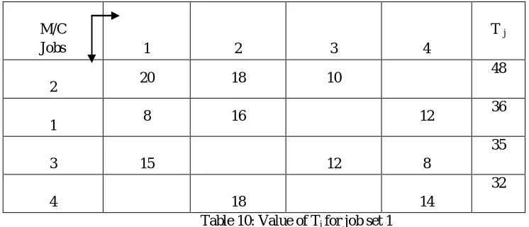
c) NEH heuristic rule for job set 1: Step1: Find the total completion time content for the all machines of each job using expression

=

Step2: Arrange the jobs in a job content list as per the decreasing values of T j

Step3: Select first two jobs from the list and from two jobs find partial sequences by interchanging the place of two jobs. Compute the total completion time (C max) value for each partial sequence and select sequence as incumbent which have small value of C max.

Step4: pick the next job and put in incumbent sequence

Ste5: if there is no job left in work content list to be added to incumbent sequence, stop go to step 4. NEH rule for job set 1: solution is constructed as follows:

Step1: jobs are arranged as per decreasing order of Tj values M/C

Jobs 1 2 3 4

T j

2 20 18 10

48

1 8 16 12

36

3 15 12 8

35

4 18 14

[image:9.612.66.547.63.150.2]

32 Table 10: Value of Tj for job set 1

Step1: taking J2&J1, we have sequence J1-J2 and J2-J1 and values of Cmax are 56 and 66 respectively as below

Job M1 M2 M3 M4

IN OUT IN OUT IN OUT IN OUT J1 0 8 8 24 24 24 24 36

J2 8 28 28 46 46 56 56 56

Table 11: Make span for sequence J1-J2

[image:9.612.97.470.406.566.2]

(10)

Technology (IJRASET)

[image:10.612.85.467.93.150.2]

549

Table 12: Make span for sequence J2-J1

Step2: choosing J1-J2 and take J3

Sequences are J1-J2--J3, J1-J3-J2 ,J3-J1-J2 and values of Cmax are 84,71 and 71 respectively as above procedure

Step3: taking J1-J3-J2& take J4 andtakingJ3-J1-J2& takeJ4

Sequences are 4-1-3-2, 1-4-3-2, 1-3-4-2, 1-3-2-4 and 4-3-2-1, 3-4-1-2, 3-1-4-2, 3-1-2-4 and values of Cmax calculated as step 1 are

71,80,80,93 and 71,77,95,93 respectively as above procedure.

Same procedure will be follow for other three job set and proceed to the FMS modeling and simulation

B. FMS Modeling Approaches

There are many FMS modeling approaches used for FMS modeling such as Mathematical modeling, computer simulation and Perti net.in the following discussion on modeling approaches, the objective is not to be present the details of modeling approaches under consideration but to identify the suitability of modeling approaches with respect to the design and operational requirement of FMS .in current system computer simulation is used for modeling the FMS system.

C. Relation of FMS System with ProModel

ProModel FMS system

location Workstation(1,2,3,4,),system buffer, machine buffer, loading and unloading system Entities Part(j1,j2,j3,j3)

[image:10.612.51.532.363.431.2]

Resources Robot And AGV

Table: Relation of FMS system with ProModel

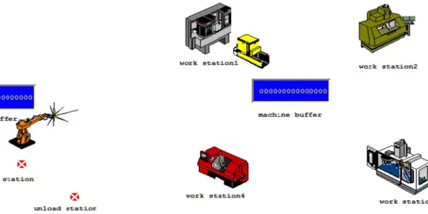
D. Building of Simulation Model

First, the modelof the FMS is created using ProModel software. The building of model is based onconsideration the inputs as processing times and incorporating the assumption, so that it represents the real problem as closely as possible. After building the entire model, connectionsare made for each types of job with each machine so that every part follows its respective route through the FMS. Then simulation is performed on the model with the set parameters. Screen shot of the simulation in progress is shown in fig.3.

Fig 3: Simulation model of FMS

Job M1 M2 M3 M4

IN OUT IN OUT IN OUT IN OUT J2 0 20 20 38 38 48 48 48

J1 20 28 38 54 54 54 54 66

[image:10.612.108.420.543.699.2]

(11)

Technology (IJRASET)

550

V. RESULTS AND DISCUSSION

A. Optimal Make span And Simulation Analysis

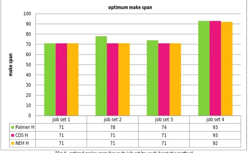
[image:11.612.64.551.161.461.2]

The results have been obtained in two partsfirst is the optimal make span foreach job set by each heuristic rules and second part is the analysis resultsof FMS using pro-model. Make span according to optimum sequencing by using the Johnson’s rule are shows by graph as below corresponding value of all the individual objectives of each job set problem with actual shop floor parameters.

Fig.4: optimal make span for each job set by each heuristic method

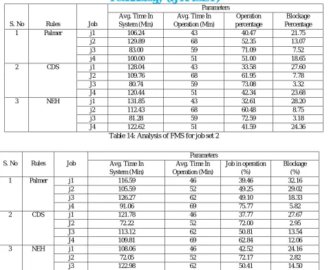
The result analysis of FMS model by used simulation approach on the basis of optimum sequencing of jobs & processing time:

S. No Rules Job

Parameters Avg. Time In

System (Min)

Avg. Time In Operation (Min)

operation percentage

Blockage Percentage 1 Palmer j1 95.72 52 54.33 11.48

j2 126.46 64 50.61 14.98 j3 108.95 51 46.81 14.88 j4 71.18 48 67.44 3.43 2 CDS j1 132.46 52 39.26 20.59

J2 160.75 64 39.81 28.34 J3 100.99 51 50.50 15.00 J4 82.88 48 57.92 5.08 3 NEH j1 108.60 52 47.88 15.18

j2 133.06 64 48.10 21.53 j3 90.35 51 56.45 3.22 J4 71.15 48 62.21 4.89

Table 13: Analysis of FMS for job set 1

job set 1 job set 2 job set 3 job set 4

Palmer H 71 78 74 93

CDS H 71 71 71 93

NEH H 71 71 71 92

0 10 20 30 40 50 60 70 80 90 100 m ak e s p an

[image:11.612.77.539.493.714.2]

(12)

Technology (IJRASET)

551

S. No Rules Job

System (Min)

Operation percentage

Blockage Percentage

1 Palmer j1 106.24 43 40.47 21.75

j2 129.89 68 52.35 13.07

j3 83.00 59 71.09 7.52

j4 100.00 51 51.00 18.65

2 CDS j1 128.04 43 33.58 27.60

J2 109.76 68 61.95 7.78

J3 80.74 59 73.08 3.32

J4 120.44 51 42.34 23.68

3 NEH j1 131.85 43 32.61 28.20

j2 112.43 68 60.48 8.75

j3 81.28 59 72.59 3.18

[image:12.612.68.546.71.463.2]

J4 122.62 51 41.59 24.36

[image:12.612.93.515.509.698.2]

S. No Rules Job

System (Min)

Job in operation (%)

Blockage (%)

1 Palmer j1 116.59 46 39.46 32.16

j2 105.59 52 49.25 29.02

j3 126.27 62 49.10 18.33

j4 91.06 69 75.77 5.82

2 CDS j1 121.78 46 37.77 27.67

J2 72.22 52 72.00 2.95

J3 113.12 62 50.81 13.54

J4 109.81 69 62.84 12.06

3 NEH j1 108.06 46 42.52 24.16

j2 72.05 52 72.17 2.82

j3 122.98 62 50.41 14.50

J4 109.22 69 63.17 12.69

Rules Job

System (Min)

Job in operation (%)

Blockage (%)

1 Palmer j1 112.06 75 66.93 12.48

j2 88.24 67 75.93 3.73

j3 119.85 57 47.56 26.48

j4 144.59 82 56.71 19.02

2 CDS j1 111.46 75 67.29 11.35

J2 88.79 67 75.45 3.41

J3 139.07 57 40.99 33.12

J4 136.37 82 60.13 16.98

3 NEH j1 120.12 75 62.44 14.39

j2 85.56 67 78.31 4.72

j3 92.21 57 58.56 18.91

[image:12.612.103.510.510.700.2]

(13)

Technology (IJRASET)

552

B. Graphs of Work Stations and Resources Utilization

Following graphs will facilitate to analyze work stations& resources utilization for different scheduling rules:

Fig.5: Work stations utilization for the jobset 1 on palmer heuristic

Fig.6. Resources utilization for the jobset 1 on palmer heuristic

(14)

Technology (IJRASET)

553

Similar graphs are generated for each job set by each heuristic rule for workstation and rersource utilization by using of pro-model simulation software.

VI. CONCLUSION

In this thesis, we have implemented three heuristic rules of scheduling which was an attempt to provide comparison and effectiveness in the solution to a scheduling. we have discussed about all the results produced by heuristic rules and tested its effectiveness using simulation approach. We have also compared the results of our proposed scheduling rules produced by simulation. After completion of comparison that can be concluded that CDS heuristic rule has performed well in many cases for that particular problem on the basis of make span minimization and workstation and resources utilization. This work is also presented the importance and significance of the shop floor parameters such as average time in system, average time in operation, operation and blockage percentage etc. It has a crucial role in efficient utilization of FMS with respect to heuristic rules of scheduling. The comparative analysis of all heuristic rules for all considered job sets is presented on the table 7.1.

Table17: Comparative analysis for heuristic rules with simulation approach:

In summary, this thesis involves developing the model and performing simulation on the FMS system and comparison and outcome of effective scheduling rule. Optimum scheduling with make span minimization are obtained by the application of three heuristic (palmer, CDS and NEH) rules for the flow shop scheduling. According to the workstation and resources utilization parameters CDS heuristic rule provide better results compare than other. Models of these arrangements of flow shop are built and simulations perform using ProModel software to validate the results by heuristic rule of scheduling. Thus it can be concluded that simulation approach can be used as an important tool for validate and make effective to scheduling of Flexible Manufacturing Systems and to understand the system behavior in a more accurate way.

TheFuture Scope in presented work can be made in future by adding other performance measures as WIP inventory, maximum lateness, tardiness etc. As a future suggestion of this article that is developing real-world integrated dynamic scheduling system by maximize the system size. That is important to combine different techniques such as operation research, artificial intelligence using expert system, together to endow the scheduling system with the required flexibility, robustness and rescheduling strategies. The work can also be extended by increasing the assumptions of the problem such as bottleneck, and machine breakdown condition

REFERENCES

(15)

Technology (IJRASET)

554

National Institute of Technology Rourkela.2009.

[2] Floorntina Alina Chircu, “Using Genetic Algorithms for Production Scheduling” BULETINUL University petrol-gaze din Ploiesti, Vol. LXII, No1/2010, pp.113-118.Mahsen bayati et.al. “Iterative scheduling algorithms IEEE INFOCOM 2007 proceeding

[3] Ezedeen kodeekha, “A new method of FMS scheduling using optimization and simulation”, proceedings 16th_{europian simulation symposium ISBN}

1-56555-286-5(book), 2004

[4] Jones,A.,& rabelo, L.C..(1998), “survey of job shop scheduling techniques”,gaithesburg, MD; technical report, nation institute of standards and technology. [5] Amar malik et.al, “Comparative Analysis of Heuristics for Make span Minimizing in Flow Shop Scheduling”,Department of Mechanical Engineering

University Institute of Engineering & Technology Maharshi Dayanand University Rohtak, Haryana, INDIA.

[6] N. Ishii and J. Talavage “A Transient-Based Real-Time Scheduling Algorithm in FMS” Int. J. Production, Research, Vol. 29,pp 2501-2520, 199 [7] Gonzalez, T. and Sen, T., 1978. “Flow shop and job shop schedules: complexity and approximations”. Operations Research 26, 36–52.

[8] Raj kumar, R. et.al. “A Bi-Criteria Approach to the m-Machine Flow Shop Scheduling Problem”, studies in informatics and control18.2(2009).127-136 [9] Garey, M.R., Johnson, D.S. and Sethi, R.R., 1976. “The complexity of flow shop and Job shop scheduling”. Operations Research 1,117–129. [10] Pinedo, M., 2005. Scheduling theory, algorithms, and system, (Prentice-Hall)

[11] Rinnooy kan, A.H.G.,(1976), “A Machine Scheduling Problem: Classification, Complexcity”,Hagueholland.

[12] Djamila Ouelhadj. Sanja Ptrovic, “A survey of dynamic scheduling in manufacturing system,” J sched (2009)12:417-431. [13] Aswani kumar dhingra, et. al., “multi objective flow shop scheduling using meta-heuristics, NIT Kurukshetra, Haryana, India [14] Gupta, J. N. D. 1988. “Two-stage, hybrid flow shop scheduling problem”, Journal of the Operational Research Society 39(4): 359-364.

[15] Santos, D. L., Hunsucker, J. L., and Deal, D. E. 1996. “An evaluation of sequencing heuristics in flow shops with multiple processors”, Computers & Industrial Engineering 30(4): 681-691.

[16] K.V.Subbaiah,et.al., “scheduling of AGVs and machines in FMS with make span criteria using sheep flock heredity algorithm.”international journal of physical sciences.vol.4(2),pp.139-148,march,2009.

[17] C saygin1 and S. Kilic2, “ Integrating Flexible Process Plans with Scheduling in Flexible Manufacturing System” Int. J Advanced Manufacturing Technology (1999) 15:pp268-280 Springer-Verlag London

[18] Felix T.S. Chan, S.H. Chung, L.Y. Chan, G. Finke, M.K. Tiwari ,“Solving distributed FMS scheduling problems subject to maintenance: Genetic algorithms approach”, Robotics and Computer-Integrated Manufacturing 22 (2006) 493–504.

[19] Safia Kedad-Sidhoum, Yasmin Rios Solis, Francis Sourd, “Lower bounds for the earliness–tardiness scheduling problem on parallel machines with distinct due dates” , European Journal of Operational Research 189 (2008) 1305–1316

[20] Moosa Sharafali , Henry C. Co , Mark Goh , “Production scheduling in a flexible manufacturing system under random demand” , European Journal of Operational Research 158 (2004) 89–102

[21] K.H. Ecker , J.N.D. Gupta, “Scheduling tasks on a flexible manufacturing machine to minimize tool change delays” , European Journal of Operational Research 164 (2005) 627–638

(16)