The Impact of Education Decentralization on Education Output: A Cross Country Study

(1)

Computer Science Theses Department of Computer Science

8-3-2007

Informative SNP Selection and Validation

Diana Mohan Babu

Follow this and additional works at: https://scholarworks.gsu.edu/cs_theses Part of the Computer Sciences Commons

Recommended Citation Recommended Citation

Mohan Babu, Diana, "Informative SNP Selection and Validation." Thesis, Georgia State University, 2007. https://scholarworks.gsu.edu/cs_theses/48

This Thesis is brought to you for free and open access by the Department of Computer Science at ScholarWorks @ Georgia State University. It has been accepted for inclusion in Computer Science Theses by an authorized

(2)

DIANA MOHAN BABU

Under the Direction of Alexander Zelikovsky

ABSTRACT

The search for genetic regions associated with complexdiseases, such as cancer or

Alzheimer's disease, is an important challenge that may lead to better diagnosis and

treatment. The existence of millions of DNA variations, primarily single nucleotide

polymorphisms (SNPs), may allow the fine dissection of suchassociations. However,

studies seeking disease association are limited by the cost of genotyping SNPs.

Therefore, it is essentialto find a small subset of informative SNPs (tag SNPs) that may

be used as good representatives of the rest of the SNPs. Several informative SNP

selection methods have been developed. Our experiments compare favorably to all the

prediction and statistical methods by selecting the least number of informative SNPs.

We proposed algorithms for faster prediction which yielded acceptable trade off. We

validated our results using the k-fold test and its many variations.

(3)

by

DIANA MOHAN BABU

A Thesis Submitted in Partial Fulfillment of the Requirements of the Degree of

Master of Science

in the College of Arts and Science

Georgia State University

(4)

Copyright by

Diana Mohan Babu

(5)

INFORMATIVE SNP SELECTION AND VALIDATION

by

DIANA MOHAN BABU

Major Professor: Alexander Zelikovsky Committee: Raj Sunderraman

Saeid Belkasim

Electronic Version Approved:

(6)

ACKNOWLEDGMENTS

I would like to take this opportunity to thank everyone who has played a significant role

during my stay at Georgia State University. I would like to thank my advisor Dr. Alex

Zelikovsky for being my guide and spending time on directing my thesis. I would also like to

thank my committee member, Dr. Raj Sunderraman and Dr. Saeid Belkasim for extending

their support and insightful comments and suggestions. A big thank you goes out to all my

friends and members of my research group Gulsah Altun, Jingwu He, Jun Zhang, Irina

Astrovskaya, Kelly Westbrooks, Qiong Cheng and Stefan Gremalschi. Special thanks thank

(7)

TABLE OF CONTENTS

ACKNOWLEDGMENTS……….. iv

LIST OF TABLES………. vii

LIST OF FIGURES……… viii

CHAPTER……….. 1. INTRODUCTION……… 1

1.1 Molecular Biology Basics………... 1

1.2 Tagging Problem………. 4

1.3 Tagging Validation……….. 5

1.4 Contributions……….. 6

1.5 Overview…...……….. 7

2. INFORMATIVE SNP SELECTION METHODS 9 2.1 Previous work in Tagging………...……… 10

2.2 STAMPA ………... 12

2.3 Tagger ……… 12

2.4 IdSelect……….……….. 13

3. TAG SELECTION BASED ON PREDICTION………... 14

3.1 Selection based on Prediction……... 14

3.1.1 STA……….. 15

3.2 Furthest SNP Extension ………... 16

3.3 Modified Furthest SNP Extension………... 17

3.4 About SNP Data set 18 3.5 Trade-off between Prediction Quality and Runtime……… 18

4. IMPROVED PREDICTION ALGORITHM………. 20

4.1 SNP Prediction Problem Formulation……… 20

4.2 Prediction of Genotypes……….. 21

4.2.1 Previous Methods 21 4.2.1.1 One – by –One Prediction ………..…... 22

4.2.1.2 Alternatives – Entropy Methods………... 22 4.2.1.3 RREF – based Prediction 23

(8)

4.2.2.1 One – after – another 28

4.2.2.2 K-Fold Cross Validation………. 29

5. STATISTICAL COVERAGE……….……… 32

5.1 r2 Computation……….………. 33

5.2 Efficiency of Tagger and MLR on MCG Data………... 34

5.3 Comparison of 3-fold cross validation on Tagger and MLR…… 35

6. CONCLUSIONS AND FUTURE WORK………. 37

7. IMPLEMENTATION………. 39

(9)

LIST OF TABLES

3.1 Comparison on Runtimes and number of Tags selected………... 18

4.1. Results of One-after-another……… 29

4.2 K-fold test performed on the prediction algorithm. K=90 is equivalent to

leave-one-out test………. 30

(10)

LIST OF FIGURES

1.1 Relationship between DNA, Genes, Chromosomes and Genome…………...… 1

1.2 Encoding SNPs for computation ……… 3

1.3 Problem formulation ………..……… 4

2.1 Problem formulation ………..………... 9

3.1 Tradeoff between runtime and number of tags for the proposed algorithms……. 19 4.1 Algorithm to use RREF for Prediction……… 26 4.2 Algorithm to calculate non-informative SNPs using coefficients……… 27 4.3. Correlation between error and number of zeros in SNP RREF……… 28 5.1 MLR-tagging for statistical covering. The shaded columns correspond to k tag

(11)

CHAPTER 1

INTRODUCTION

1.1 Molecular Biology basics

DNA (Deoxyribonucleic acid) is one of the building blocks of life that carries the genetic

information in living things. It has a double helix structure which consists of two

complementary strands of nucleotides. Each of the two strands serves as a template for

synthesis of a new DNA strand during replication. Information in DNA is organized into

genes which are packaged into chromosomes. All chromosomes taken together form an

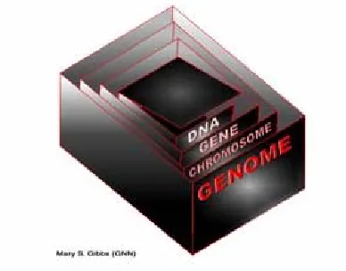
[image:11.612.218.412.321.473.2]

organism's Genome and affect specific characteristics of the organism.

Figure 1.1. Relationship between DNA, Genes, Chromosomes and Genome

Imagine these relationships as a set of Chinese boxes nested one inside the other

(Figure1.1). The largest box represents the genome. Inside it, a smaller box represents the

chromosomes. Inside that is a box representing genes, and inside that, finally, is the

smallest box, the DNA. In short, the genome is divided into chromosomes, chromosomes

contain genes, and genes are made of DNA.

Genes are made of DNA, and so is the genome itself. A gene consists of enough DNA to

(12)

is the molecule that is the hereditary material in all living cells. The bases found in DNA

come in four varieties: adenine, cytosine, guanine, and thymine—often abbreviated as A,

C, G, and T, the letters of the genetic alphabet.

Genes are found on chromosomes and are made of DNA. Different genes determine the

different characteristics, or traits, of an organism. In the simplest terms (which are

actually too simple in many cases), one gene might determine the color of a bird's

feathers, while another gene would determine the shape of its beak.

A chromosome is a package containing a chunk of a genome—that is, it contains some of

an organism's genes. Chromosomes help a cell to keep a large amount of genetic

information neat, organized, and compact.

Human beings have 46 chromosomes (23 from mother and 23 from father). Diploid

organisms, like human beings, have a pair of nearly identical chromosomes. A copy of

each chromosome is called a haplotype. Data consisting of pairs of haplotypes is called a

genotype. Genome difference between any two people is about 0.1% of genome. These

differences are Single Nucleotide Polymorphisms (SNPs). More than 4 million SNP's

have been identified and the information has been made publicly available. SNPs may

occur in both coding (gene) and non-coding regions of the genome. Many SNPs have no

effect on cell function, but they could predispose people to disease or influence their

(13)

[image:13.612.113.516.67.302.2]

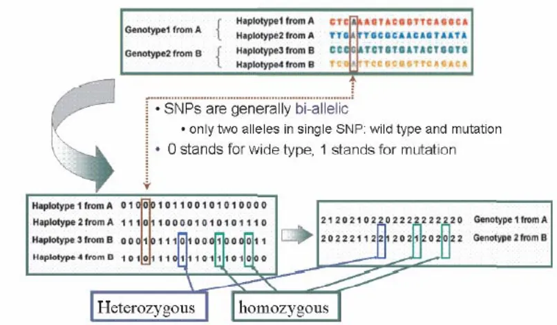
Figure 1.2. Encoding SNPs for computation

A SNP is a specific location in our DNA where different people have different DNA

bases. For example, at a specific point in your DNA you may have the DNA base

cytosine (C) and another person may have the DNA base thymine (T). SNPs are

bi-allelic, so if you possess two copies of C or two copies of T at this location, one on each

of your pair of chromosomes, you are homozygous. If you possess a C and T at this

location you are heterozygous. Homozygous is represented as 0 or 1 (depending on its

value) whereas heterozygous is represented as 2 in the genome (Figure 1.2).

The major allele is considered to be the wild type while the minor allele is considered to

be the mutation. Hence, SNPs portray the genetic differences among people which will

(14)

1.2 Tagging Problem

The search for genetic regions associated with complexdiseases, such as cancer or Alzheimer's

disease, is an importantchallenge that may lead to better diagnosis and treatment. Theexistence

of millions of DNA variations, primarily single nucleotidepolymorphisms (SNPs), may allow

the fine dissection of such associations. However, studies seeking disease association are

limited by the cost of genotyping SNPs. Therefore, it is essentialto find a small subset of

informative SNPs (tag SNPs) that maybe used as good representatives of the rest of the SNPs

[1].

In order to handle data with huge number of SNPs, one can extract informative SNPs that

can be used for (almost) lossless reconstructing of all other SNPs. To avoid information

loss, index SNPs are chosen based on how well the other non-tag SNPs can be reconstructed.

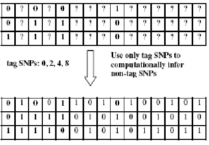
The corresponding informative SNP selection problem (ISSP) can be formulated as

[image:14.612.217.422.411.553.2]

follows (Figure 1.3).

Figure 1.3. Problem formulation

Given a sample S of a population P of individuals (either haplotypes or genotypes) on m

SNPs, select positions of k (k < m) SNPs such that for any individual, one can predict

non-selected SNPs from these k selected SNPs. The Multiple Linear Regression based

(15)

informative SNPs minimizing the prediction error measured by the number of incorrectly

predicted SNPs. The number of tags (informative SNPs) k depends on the desirable data

size. More tags will keep more genotype information while fewer tags allow deeper analysis

and search.

Using statistical methods, the informative SNPs are captured using the correlation

coefficient r 2. This is done by selecting the SNPs in the sample which are able to predict

other SNPs in the sample with a correlation of at least a certain amount. For example, if

r2>0.8, each non-tag SNP should be predicted with an accuracy of at least 80%. If the value

of r2 =1, it shows that the two SNPs are identical, if r2 =0 it shows no correlation at all.

The effectiveness of the tags varies with the number of tags chosen and the desired

correlation set. If the desired correlation is high, the number of tags selected is highly

effective. If the number of tags selected is too little, the accuracy is low. The more the

number of tags used, the better the prediction. Our intention is to chose the optimal number

of tags with reasonably high correlation in order to achieve the best results.

1.3 Tagging Validation

In MLR-tagging [7], the validation has been done using the leave-one-out test. In this

method, one individual is removed from the sample file and its value is predicted using the

tags found. The predicted value is then compared with the original value of that individual

and the accuracy is determined. This process is repeated till all the individuals have been

predicted.

Keeping in mind that these tags will be used to predict many unknown SNPs, for which

the accuracy cannot be measured, we decided to perform the k-fold test. In this method, the

sample population is divided into k equal parts. One kth_{of the file is predicted based on}

(k-1)/k parts of the file. This is done for all the parts and the average accuracy is calculated. This

(16)

prediction accuracy increases. As the number of SNPs to be predicted increases, the

prediction accuracy decreases.

1.4 Contributions

A lot of work was done in the various methods of informative SNP selection. We

started with the prediction based methods and then moved on to statistical methods for

informative SNP selection. Statistical methods were found to perform better giving high

accuracy.

We propose two new algorithms for selection based on prediction – Furthest SNP

Extension and Modified FSE. The intuition behind these algorithms was based on the

TSP heuristic analogy of furthest neighbor extension. It seeks to find the furthest

distance that a point can be from a graph. In this algorithm, the furthest two points

are joined. The next point selected is furthest from both the selected points. Even

though our algorithm does not directly use prediction; in a way, the largest distance

represents the SNPs that are least correlated. This shows that prediction is also

considered in the form of the distance values, even though it is not the focus of our

algorithms. We found that Furthest SNP Extension has the best trade off between

runtime and number of informative SNPs selected.

In Section 4, we propose an improved prediction algorithm where the prediction

focus of the problem was to improve the prediction capability in spite of longer

runtimes and more tags. In our method, one individual is hidden from the sample genotype

and its value is predicted. The predicted value is compared against the actual value. This

(17)

uses a novel approach of using the previously predicted value in the prediction of its neighbors.

We also performed the k-fold cross validation to test our method.

In Section 5, statistical covering is discussed. Initially MLR [7] did not perform up to the

mark as Tagger [3]. We tweaked the formula used to calculate the correlation coefficient (r2_{) and}

gained better performance than Tagger [3].When predicting a non-tag SNP, the

MLR-tagging method accumulates information about all tag SNPs resulting in significantly

higher prediction accuracy with the same number of tags than for the previously known

tagging methods. We confirmed our results using 3-fold cross-validation.

1.5 Overview

Chapter 2 talks about the current methods used for informative SNP selection. The

methods discussed are IdSelect [4], STAMPA [5], and Haploview (specifically the Tagger

module) [3]. IdSelect [4] uses the greedy approach to select tag SNPs. STAMPA [5] uses

dynamic programming to select the tags and calculate best prediction score. Tagger [3] uses

statistical methods combined with the greedy approach to choose tags.

Chapter 3 proposes different algorithms considered for tag selection. STA [6] is used

as the benchmark in terms of trade off between runtime and accuracy. The main focus in

this experiment is the time taken. Two algorithms with faster runtimes are analyzed. On an

average, it is found that as the runtime decreases the number of informative SNPs selected

increases.

Chapter 4 proposes an improved prediction algorithm based on linear reduction method.

The newly predicted non-tag SNP is used as a tag in the prediction of the next SNP. We

propose an improved prediction algorithm where the prediction focus of the problem

was to improve the prediction capability in spite of longer runtimes and more tags.

(18)

with Haploview [3], we reexamine the formula and data being used to calculate r2. Upon

modifying the algorithm, we were able to achieve better results than Haploview [3] for our test

sets.

(19)

CHAPTER 2

INFORMATIVE SNP SELECTION METHODS

In order to handle data with huge number of SNPs, one can extract informative SNPs that

can be used for (almost) lossless reconstructing of all other SNPs. To avoid information

loss, index SNPs are chosen based on how well the other non-tag SNPs can be reconstructed.

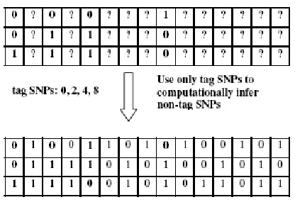
The corresponding informative SNP selection problem (ISSP) can be formulated as

[image:19.612.215.423.285.431.2]

follows (Figure 1.3).

Figure 2.1. Problem formulation

SNPs, select positions of k (k < m) SNPs such that for any individual, one can predict

non-selected SNPs from these k selected SNPs. The Multiple Linear Regression based

MLR-tagging algorithm [7] solves the optimization version of ISSP which asks for k

informative SNPs minimizing the prediction error measured by the number of incorrectly

predicted SNPs. The number of tags (informative SNPs) k depends on the desirable data

size. More tags will keep more genotype information while fewer tags allow deeper analysis

and search.

(20)

This is done by selecting the SNPs in the sample which are able to predict other SNPs in the

sample with a correlation of at least a certain amount. For example, if r2>0.8, each non-tag

SNP should be predicted with an accuracy of at least 80%.

The effectiveness of the tags varies with the number of tags chosen and the desired

correlation set. If the desired correlation is high, the number of tags selected is highly

effective. If the number of tags selected is too little, the accuracy is low. The more the

number of tags used, the better the prediction. Our intention is to chose the optimal number

of tags with reasonably high correlation in order to achieve the best results.

2.1 Previous work in Tagging

Previous research on tag SNP selection has explored both lossless and lossy methods.

Lossless methods select a set of tag SNPs that capture 100% of the haplotypic variation

in the sample population. Lossy methods typically select fewer tags than lossless

methods, but with some tolerated amount of information loss.

Aviitzhak et al. [4] presented a method for selecting tags which can be used in both a

lossless and a lossy manner. The central idea behind both their lossless and lossy methods

is to eliminate tags that contribute the least to the Shannon entropy for the haplotype set.

First, identical columns and complimentary columns are eliminated, then they eliminate

columns that do not reduce the number of unique rows. They note that selecting a

maximal linearly independent set of column vectors would miss opportunities to

eliminate complimentary SNPs and illustrate that by the 2-by-2 identity matrix. Their

lossless method reduces by 25% and 36% the number of SNPs describing the haplotype

diversity within an African-American and Caucasian population, respectively.

Zhang et al. [51] introduced a block-based, dynamic programming algorithm for

haplotype inference that is capable of reconstructing 90% of the original data using only

(21)

algorithm for haplotype inference, and as a result, provided a method of performing

association studies directly on genotype data.

Sebastiani et al. [43] described a lossless method called BEST (Best Enumeration of

SNP Tags) for identifying a minimal set of tag SNPs from haplotype data. BEST selects

tags by determining if a candidate tag is a boolean function of SNPs already chosen as

tags. The BEST method selected 14% of SNPs as tags from an African- American

population and 10% from an European-American population by considering individual

genes each ranging from 5 to 229 SNPs in length. However, its effectiveness on a

genome-wide scale is still unproven. According to their method, 95% of tags selected

from the European-American population were also selected from the African-American

population, which provides evidence for the a genetic bottleneck event that occurred long

ago as hominids migrated out of Africa to settle Europe and Asia.

Halldorson et al. [23] defined the informative ness measure of how well a set of tags

describes a haplotype sample. Both the informativeness measure, as well as their tag SNP

selection method consider a graph whose vertices are SNPs; an edge is placed between to

SNPs if one SNP can be used to reliably predict the other. Their method seeks the set of

SNPs that maximizes the informativeness measure on the haplotype data. The method

can achieve prediction rates of 90% based on only 20% of SNPs. Halldorsson's method

differs from the others in that it is a block-free method. Block-based methods are

restricted to identifying tags only within local contiguous sequences of SNPs where the

haplotype diversity is low. Block-free methods have the capability to identify tags across

an entire genome. Like Halldorsson's method, the linear reduction method we propose is

a block-free method.

Lee et al. [34] introduce BNTagger, a new method for tagging SNP selection, based

(22)

(BNs), their system aims to select a subset of independent and highly predictive SNPs.

For example, BNTagger uses 10% tags to reach 90% prediction accuracy. However,

BNTagger comes at the cost of compromised running time. Its running time varies from

several minutes (when the number of SNPs is 52) to 2-4 hours (when the number is 103).

Our tagging problem formulations and above approaches do not take into account

haplotype frequency when selecting a tag SNPs.

2.2 STAMPA

Halperin et al. [1] describes a new method STAMPA for SNP prediction and tag selection.

A SNP is predicted by inspecting the two closest tag SNPs from both sides; the value of the

unknown SNP is given by a majority vote over the two tag SNPs. They use dynamic

programming to select tags to reach best prediction score. Their methods are compared with

idSelect and HapBlock on a variety of data sets, and could predict with 80% accuracy the SNPs

in the daly dataset[17] using only 2 SNPs as tags. In general, this problem is computationally

difficult and the runtime of an exact algorithm may become prohibitively slow. Therefore, one

can use heuristics for the selection of k tags following Halperin et al.[1] who compare relatively

slow STAMPA with a fast random tag selection.

2.3 Tagger[3]

De Bakker et. all [3] describe how to select the informative SNPs using the SNPs that

surround it. They claim that SNPs that are in close distance are highly correlated and tag SNPs

should be picked from this pool (One tag from each pool) of highly correlated SNPs. A simple

and conservative approach is used to select tag SNPs from a subset of non redundant SNPs from

the genotype data such that every common allele either is perfectly genotyped or is identical

(23)

them. They select random tags and test them using the 2 X 2 χ2 test. If all SNPs are not covered,

they find another set of informative SNPs. Similarly they run multiple tests on a set of tags and

try to find the set that passes the most number of tests. Also test are performed with 1 degree of

freedom to prevent over fitting. Sometimes, if a combination of SNPs can be used for prediction,

this combination is used as a tag.

2.4 idSelect [13]

IdSelect, developed by Carlson et al.[13], used a greedy approach for tag SNP selection.

They developed a greedy algorithm to identify subsets of tag SNPs for genotyping, selected

from all SNPs exceeding a specified MAF threshold. Starting with all SNPs above the MAF

threshold, the single site exceeding the threshold with the maximum number of other sites above

the MAF threshold is identified. This maximally informative site and all associated sites are

grouped as a bin of associated sites. Not all SNPs within the bin are interchangeable, because

pairwise association is not an associative property: if r2 exceeds the threshold for SNP pairs A/B

and B/C, r2 for SNP pair A/C might not exceed the threshold. Thus, because the bin is initially

ascertained using a single SNP, all pairwise r2 within bin are re-evaluated, and any SNP

exceeding threshold r2 with all other sites in the bin is specified as a tag SNP for the bin. Thus,

one or more SNPs within a bin are specified as tag SNPs, and only one tag SNP would need to

be genotyped per bin. The informative SNP can be selected for assay on the basis of genomic

context (coding vs. noncoding or repeat vs. unique), ease of assay design, or other user-specified

criteria. The binning process is iterated, analyzing all as-yet-unbinned SNPs at each round, until

all sites exceeding the MAF threshold are binned. Each bin is reported as a set of all SNPs in the

bin as well as the subset of tag SNPs within the bin, each of which is above the r2 threshold with

all other SNPs in the bin. If an SNP does not exceed the r2 threshold with any other SNP in the

(24)

CHAPTER 3

TAG SELECTION BASED ON PREDICTION

In tag SNP selection, speed is an important issue. If the tags take too long to compute, it

becomes a more expensive option to tag SNPs. In some cases the informative SNP values may

not be as important as the time taken for selection. Keeping this trade-off in mind two

algorithms are proposed.

The intuition behind the following algorithms was based on the TSP heuristic

analogy of furthest neighbor extension. It seeks to find the furthest distance that a

point can be from a graph. In this algorithm, the furthest two points are joined. The

next point selected is furthest from both the selected points. In this way, all points

are selected based on largest distance between them. Even though our algorithm

does not directly use prediction; in a way, the largest distance represents the SNPs

that are least correlated (r2 is close to 0). This shows that prediction is also

algorithms.

3.1 Selection based on Prediction

Most informative SNP selection methods place more importance on the prediction

accuracy obtained over the runtime of the program. This is evident in most prediction methods

used today. We will consider idSelect [13] and STA [6], two methods with slow runtimes

which place a great deal of importance on prediction accuracy.

IdSelect, developed by Carlson et al.[13], used a greedy approach for tag SNP selection.

They developed a greedy algorithm to identify subsets of tag SNPs for genotyping, selected

(25)

threshold, the single site exceeding the threshold with the maximum number of other sites above

the MAF threshold is identified. This maximally informative site and all associated sites are

grouped as a bin of associated sites. Not all SNPs within the bin are interchangeable, because

pairwise association is not an associative property: if R2 exceeds the threshold for SNP pairs A/B

and B/C, R2 for SNP pair A/C might not exceed the threshold. Thus, because the bin is initially

ascertained using a single SNP, all pairwise R2 within bin are re-evaluated, and any SNP

exceeding threshold R2 with all other sites in the bin is specified as a tag SNP for the bin. Thus,

one or more SNPs within a bin are specified as tag SNPs, and only one tag SNP would need to

be genotyped per bin. The tag SNP can be selected for assay on the basis of genomic context

(coding vs. noncoding or repeat vs. unique), ease of assay design, or other user-specified criteria.

The binning process is iterated, analyzing all as-yet-unbinned SNPs at each round, until all sites

exceeding the MAF threshold are binned. Each bin is reported as a set of all SNPs in the bin as

well as the subset of tag SNPs within the bin, each of which is above the r2 threshold with all

other SNPs in the bin. If an SNP does not exceed the r2_{threshold with any other SNP in the}

region, it is placed in a singleton bin.

3.1.1 Stepwise Tag Selection Algorithm (STSA) [7]

The Stepwise Tag Selection Algorithm (STSA) [7] starts with the best tag t0, i.e., tag that

minimizes error when predicting with Akall other tags. Then STSA finds such tag t1 which

would be the best extension of {t0}and continue adding best tags until reaching the set of tags

of the given size k. STSA produces hereditary set of tags, i.e., the chosen k tags contain the

chosen k-1 tags. This hereditary property may be useful in case if the set of tags can be

extended. The runtime of STSA is O(knmT), where T is the runtime of the prediction

algorithm. Note that for statistical covering, STSA is equivalent to the greedy algorithm

(26)

3.2 Furthest SNP Extension

The intuition behind the following algorithms was based on the TSP heuristic

analogy of furthest neighbor extension. It seeks to find the furthest distance that a

point can be from a graph. In this algorithm, the furthest two points are joined. The

next point selected is furthest from both the selected points. In this way, all points

are selected based on largest distance between them. Even though our algorithm

does not directly use prediction; in a way, the largest distance represents the SNPs

that are least correlated (r2 is close to 0). This shows that prediction is also

algorithms.

In this algorithm the tag SNPs are calculated based on the distance between them (Euclidian

or r2). A SNP s1 is picked that covers maximum number of SNPs. The next SNP s2 picked is

the farthest SNP from s1, that is, distance between s1 and s2 is the maximum as opposed to

distance between s1 and any other SNP. s1 and s2 are tested to see how many SNPs are

covered. If all SNPs are not covered, add SNP s3 such that it is at maximum distance from s1

after s2. This process is carried out until all SNPs are covered. The algorithm is demonstrated

below.

Input: Sample Population S with n genotypes m SNPs each

Output: Set T of tag SNPs

1. Find T={t1} where t1 covers most number of SNPs

2. Calculate the distance matrix MD from each SNP to t1.

3. While SU<> empty, SU subset of SNPs from S which are not covered by T do

3.1. s1 is added to T if distance(s1,T)>max, s1 from SU

(27)

This algorithm was found to be the moderately fast. The tags predicted were not of the best

quality, but they were acceptable.

3.3 Modified Furthest SNP Extension

Using this method, the tag SNPs are calculated based on the distance between them (Euclidian

or r2). A SNP pair (s1, s2) is initially picked such that the distance between s1 and s2 is maximal

between all SNPs. The next SNP s3 is added such that it is at maximal distance from s1 and s2.

This process is carried on until all the SNPs are covered. The algorithm is described below.

Input: Sample Population S with n genotypes m SNPs each

Output: Set T of tag SNPs

1. Calculate the distance matrix MD from each SNP to s1.

2. Find SNP pairs s1 and s2 that are maximum distance apart from each other. Add s1 and s2 to

tags T.

3. While SU<> empty, SU subset of SNPs from S which are not covered by T do

3.1. s3 is added to T where distance(s1,T)>max, s3 from SU

4. Output T

This experiment was conducted using the same test sets and values as the others. The results are

calculated in the shortest time. The predicted tags were acceptable as they were not too much or

too sparse. This algorithm was found to be the fastest. The tags predicted were not of the best

(28)

3.4 About SNP Data set

We ran our test on the data sets provided to us by Medical College of Georgia

(MCG). They provided us with the genotype data of certain genes that they wanted to

study. The size of the largest set was 71 SNPs. The original size was much larger (130

SNPs), but we only wanted to consider those SNPs with minor allele frequency (MAF)

over 5%. The r2 (correlation coefficient) was kept at 0.8.

3.5 Trade-off between Prediction Quality and Runtime

In this section we discuss our findings. It was found that quality decreases with increase in

runtime. However, the quality does not drastically decrease in all cases. The furthest SNP

extension method and the modified FSE do not a lot of runtime difference. Modified FSE was

found to be faster only by a few milliseconds.

Runtime (in seconds)

Data Set Statistical Tagging

Furthest SNP Extension

(FSE) Modified FSE

# of

Tags Runtime

# of

ADIPOQ-AA 11 5 12 1.3 12 1.1

ADIPOQ-EA 10 5.5 11 1.68 11 1.34

ADIPOR1-AA 10 5.1 11 1.73 11 1.41

ADIPOR1-EA 6 1.2 7 0.7 6 0.6

ADIPOR2-AA 15 35 18 24.2 23 22

[image:28.612.108.545.390.535.2]

ADIPOR2-EA 9 31.7 11 20.1 14 18

Table 3.1. Comparison on Runtimes and number of Tags selected

From Table 3.1 we can see that Furthest SNP Extension is the most optimal algorithm in

terms of the trade-off between runtime and the number of tags selected. The runtimes are given in

milliseconds. The last two data sets, which are also the largest, have the longest runtime. It

should be noted that as the file size increases, the runtime increases. In these cases, the runtime of

(29)

Tradeoff between Runtime and Number of Tags

0 5 10 15 20 25

0 10 20 30 40

Runtime

N

u

m

b

e

r of

Ta

g

s Statistical Tagging

Furthest SNP Extension (FSE)

[image:29.612.132.501.69.272.2]

Modified FSE

Figure 3.1. Tradeoff between runtime and number of tags for the proposed algorithms

Figure 3.1 shows a graph displaying the tradeoff between runtime and number of tags

selected for each algorithm. It can be noticed that the runtime is least for modified FSE, which

also selects the most number of tags. Furthest SNP Extension yields the optimal result as the

runtime is significantly decreased as compare to statistical tagging, while the number if tags

(30)

CHAPTER 4

IMPROVED PREDICTION ALGORITHM

This chapter talks about the various prediction methods that have been used and how we

improved upon them. There are many methods that can be used for SNP prediction. Most of

them use the one – by – one prediction. In this method, one individual is hidden from the

sample genotype and its value is predicted. The predicted value is compared against the actual

value. This process is carried out until all the individuals have been predicted. Our method of

prediction uses a novel approach of using the previously predicted value in the prediction of its

neighbors.

4.1 SNP Prediction Problem Formulation

SNP prediction calculates the values of the unknown SNPs using the tags that have

been determined for a given sample. The prediction may also be carried out on known

values to determine the accuracy of the method used. The prediction problem can be

formulated as follows:

SNPs and positions of k (k < m) tag SNPs, one can predict non-selected SNPs from these

k selected SNPs with good accuracy.

Given the full pattern of all haplotypes in a small population sample, find the

minimum number of tag SNPs and a method for reconstructing each haplotype in the

entire population from these tags.

There are many methods to do prediction such as one-by-one prediction, simultaneous

prediction and one-after-another prediction. Simultaneous prediction is done using entropy

methods wherein random SNPs are picked at a time and their values are predicted together.

(31)

The Multiple Linear Regressionbased MLR-tagging algorithm [7] solves the optimization

version of ISSP which asks for k informative SNPs minimizing the prediction error measured

by the number of incorrectly predicted SNPs. The number of tags (informative SNPs) k

depends on the desirable data size. More tags will keep more genotype information while

fewer tags allow deeper analysis and search.

4.2 Prediction of Genotypes

There are many methods to do prediction such as one-by-one prediction, simultaneous

prediction and one-after-another prediction. Simultaneous prediction is done using entropy

methods wherein random SNPs are picked at a time and their values are predicted together.

Most common methods use one-by-one prediction like STAMPA [1] and MLR [7].

4.2.1 Previous Methods

The methods used were one-by-one prediction wherein one value is predicted at a

time. Entropy methods were proposed where multiple values could be predicted

simultaneously. Another method is based on finding the RREF of the training set to test

(32)

4.2.1.1 One-by-One prediction

One-by-One prediction, as the name suggests, predicts one value at a time. So, if n

SNPs are to be prediction it would require n runs to predict all the SNPs. This method is

time consuming but highly accurate. Due to the time it takes, it is unsuitable for large

data sets. One-by-one prediction is the most commonly implemented method for

informative SNP prediction. STAMPA and MLR are based on this theory.

The Multiple Linear Regressionbased MLR-tagging algorithm [7] solves the optimization

version of ISSP which asks for k informative SNPs minimizing the prediction error measured

by the number of incorrectly predicted SNPs. The number of tags (informative SNPs) k

depends on the desirable data size. More tags will keep more genotype information while

fewer tags allow deeper analysis and search

4.2.1.2 Alternatives - Entropy Methods

A more complex method of prediction is by predicting multiple SNPs

simultaneously. The tags of the known SNPs are compared with the informative

(33)

informative SNP values (least hamming distance) to the unknown individual is

considered to be the best fit. The non-informative SNP values of this sample

genotype is copied and set as the values for the unknown SNPs in the genotype we

are predicting. This method is considered to be one of the least accurate methods as

it is extremely rare that the values of the unknowns will match with those of the

sample population. Experiments carried out using this method yielded undesirable

results.

The advantage of this method is the speed. As it uses known values from the

training data the speed of prediction is much faster as compared to any other

method.

4.2.1.3 RREF – based Prediction

Initially, the actual Euclidian distance was calculated between the informative SNPs and

the remaining SNPs. This is not an accurate measure as it does not give us any information

about the linear combination of SNPs. It is found that a linear combination of the

informative SNPs can be used to predict the remaining SNPs.

We found out that the best way to find the linear independent SNPs (informative SNPs

or tags) is by reducing the population matrix into reduced row echelon form.Typically, in

genetic sequences derived from human haplotypes, the number of sites is much larger than the

number of individuals. Because of such disproportion, many columns corresponding to SNP sites

are similar. Indeed, the number of equivalent sites in real data is considerably large. The

0-1-column-site si is equivalent to the site sj if either si and sj are the same, si = sj, or si is

complimentary to sj(i.e., sibecomes sjafter each 0 is replaced with 1 and each 1 is replaced with

0). It is common to keep only one site out of several equivalent sites since they do not carry any

(34)

In general, if one column-site can be restored from several other columns, then it can be

dropped without loss of information. We consider restoration of one column-site using a linear

combination of other column-sites.

One can also explore linear dependency of rows-haplotypes rather than columns-SNPs. Then

linear dependency in (-1,1)-notations can be used for classification of recombination. Assume that

in the given population all recombination happen at a limited number of hotspots. Assume further

that each hotspot occupies a DNA segment between two consecutive SNPs. If initially there are

only two haplotypes a and b, then by repeatedly recombining a and b at g different hotspots, one

can potentially obtain as much as 2g+1_{different haplotypes.}

Let H be a set of haplotypes obtained from two haplotypes by recombination events at g

hotspots. Then the number of linearly independent rows-haplotypes is at most g+2, i.e., the linear

rank of H , rank(H ) ≤ g+2.

Our basic linear reduction method for tagging assumes that if there is a linear dependency

between certain SNPs in the given sample H, then the same dependency is likely to hold for these

SNPs in the entire population P. Based on this assumption, we suggest (i) to find linear

dependencies in the sample, (ii) extract linear independent SNPs using them as tags, and (iii)

reconstruct the values of non-tag SNPs based on values of tag SNPs and linear dependencies

found in the sample H.

Formally, our basic linear reduction method for tagging consists of the following steps:

• From the sample haplotype matrix H, extract the maximum number r = rank(H) of

linearly independent columns-SNPs T(H) = {Ht1……Htr} forming a basis of

(35)

• For each column-SNP Hj; j = 1…..m in H, find a unique representation of Hj as a linear

combination of tag SNPs

Hj =

∑

= r

i1

αi,j Hti

• Output the positions {t1………tr} of tag SNPs of T(H) and the matrix F =(αi,j) of

coefficients of linear combinations.

The suggested linear reduction method can be implemented very efficiently. Applying

O(n2m) Gauss-Jordan elimination, we can transform the n x m matrix H into the reduced row

echelon form R which will have exactly r = rank(H) nonzero rows. The r tag SNPs formed by

linearly independent column-sites corresponding to nonzero rows can be easily found from R. Let

F be the matrix R in which zero rows are dropped, so F is an r£m matrix. Then for any haplotype

h with the tag SNP values hr, the predicted reconstruction h= f (hr) equals

h= hrX F

The haplotype information is spread all over the haplotype length and the first r linearly

independent columns do not necessarily give the best choice of tags. Finally, we compare the

following variations of the initial method:

(i) Linear Reduction (LR), where the SNPs are processed in the order as in H and

(ii) Randomized Linear Reduction (RLR), which is LR where H is preprocessed by randomly

permuting columns-SNPs.

(iii) RLR with postprocessing (RLRP), which is RLR where unresolved SNPs are

(36)

When the required number of tags k is specified, then it may not necessarily coincide with

the linear rank of the sample matrix H. Figures 1 and 2 show how to adjust RLRP = RLRP(k)

for required number of tags k. In case when the required number of tags k is less than the

linear rank of H, we suggest to reduce the sample to k linear independent haplotypes. We

found that it is better to choose the most representative haplotypes, i.e., haplotypes that can

predict all others with the least number of errors (Figure 4.1).

(37)

In case when the required number of tags k is more than the linear rank r of H, we suggest

to add more SNPs to the initial r tags and form k¡r+1 different reconstruction matrices

corresponding to k – r + 1 different r-subsets of k tags. In the reconstruction phase, we

aggregate the information from all k – r + 1 reconstructions each based on different tag

subsets. The aggregation is suggested to be done by “voting”: the value of -1 (respectively, 1)

is assigned if majority of k – r + 1 reconstructions suggests -1 (respectively, 1) (Figure 4.2).

(38)

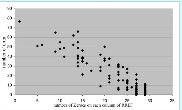
The number of zeros for SNPs in the RREF of the genotypes indicates the error in

the prediction column. The more the number of zeros in a column, the better is the

prediction obtained using that SNP (Figure 4.3). The SNPs with the largest number of

[image:38.612.176.473.179.359.2]

zeros in their RREF are added to the list of tags.

Figure 4.3. Correlation between error and number of zeros in SNP RREF.

4.2.2 Our Proposed Method

Since the predictions so far were not very good, we decided to try a novel approach by

adding the last predicted SNP to the set of tags. We used RREF based prediction algorithm

and modified it to use non-tags in the prediction of its neighbors.

4.2.2.1 One-after-Another Prediction

The idea behind this algorithm is solely focused on improving the prediction and so we

are unconcerned about the runtime. One-after-another prediction uses the most recently

predicted value as a tag in the prediction of its neighbors. As it has been found that SNPs that

are close to one another are highly correlated, this method is found to be very effective.

Considering that error is propagated, we check the accuracy of the predicted SNP before

0 10 20 30 40 50 60 70 80 90

0 5 10 15 20 25 30 35

number of Zeroes on each column of RREF

number

of

er

ro

(39)

using it in the prediction of its neighbor. If a SNP is not predicted with high accuracy, it is not

considered in the prediction of its neighbors. This minimizes error propagation.

We use RREF-based prediction in this algorithm. The error in prediction using a given

SNP is decided by the number of zeros in its RREF column. This algorithm was run on all

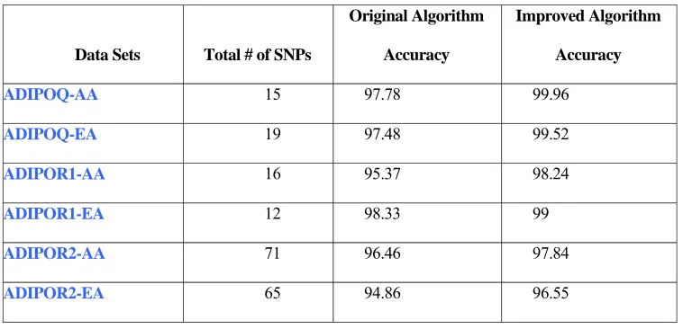
the datasets and we noticed that the accuracy increased as expected. (Table 4.1)

Data Sets Total # of SNPs

Original Algorithm

Accuracy

Improved Algorithm

Accuracy

ADIPOQ-AA 15 97.78 99.96

ADIPOQ-EA 19 97.48 99.52

ADIPOR1-AA 16 95.37 98.24

ADIPOR1-EA 12 98.33 99

ADIPOR2-AA 71 96.46 97.84

[image:39.612.109.488.195.378.2]

ADIPOR2-EA 65 94.86 96.55

Table 4.1. Results of One-after-another.

4.2.2.2 K-Fold Cross Validation

Cross-validation and bootstrapping are both methods for estimating generalization error

based on "resampling". It is the practice of partitioning a sample of data into subsets such

that the analysis is initially performed on a single subset, while the other subset(s) are

retained for subsequent use in confirming and validating the initial analysis. The initial

subset of data is the training set; the other subset(s) are called validation or testing sets.

In k-fold cross-validation, we divide the data into k subsets of (approximately) equal

size. We use each part as a test and the remaining k-1 parts as training. This procedure is

done for each part and the perdiction accuracy is noted k times. The average of the k

(40)

data set, it is called leave-one-out.

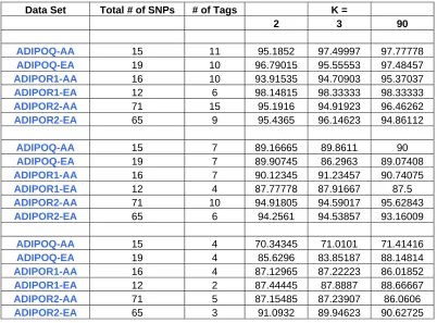
Table 4.2 summarizes our k-fold cross validation. As we can see, the prediction

accuracy increases as the size of the training set increases.

Data Set Total # of SNPs # of Tags K =

2 3 90

ADIPOQ-AA 15 11 95.1852 97.49997 97.77778

ADIPOQ-EA 19 10 96.79015 95.55553 97.48457 ADIPOR1-AA 16 10 93.91535 94.70903 95.37037 ADIPOR1-EA 12 6 98.14815 98.33333 98.33333

ADIPOR2-AA 71 15 95.1916 94.91923 96.46262

ADIPOR2-EA 65 9 95.4365 96.14623 94.86112

ADIPOQ-AA 15 7 89.16665 89.8611 90

ADIPOQ-EA 19 7 89.90745 86.2963 89.07408

ADIPOR1-AA 16 7 90.12345 91.23457 90.74075

ADIPOR1-EA 12 4 87.77778 87.91667 87.5

ADIPOR2-AA 71 10 94.91805 94.59017 95.62843

ADIPOR2-EA 65 6 94.2561 94.53857 93.16009

ADIPOQ-AA 15 4 70.34345 71.0101 71.41416

ADIPOQ-EA 19 4 85.6296 83.85187 88.14814

ADIPOR1-AA 16 4 87.12965 87.22223 86.01852

ADIPOR1-EA 12 2 87.44445 87.8887 88.66667

ADIPOR2-AA 71 5 87.15485 87.23907 86.0606

[image:40.612.109.511.191.488.2]

ADIPOR2-EA 65 3 91.0932 89.94623 90.62725

Table 4.2. K-fold test performed on the prediction algorithm. K=90 is equivalent to leave-one-out test.

In this test we checked the prediction accuracy using the prediction algorithm. We

checked how the accuracy varies as we decrease the number of tags used in prediction.

The number of tags used is proportional to the file size as well. If we decrease the

number of informative SNPs drastically for a large file, the prediction accuracy

decreases drastically. In medium sized files the decrease is less obvious. The size of the

training set is also plays a big factor in the accuracy. As the size of the training set is

(41)

as the leave-one-out test. The most accurate test in this table, in terms of how we will

(42)

CHAPTER 5

STATISTICAL COVERAGE

There have been many statistical methods proposed for finding informative SNPs. We

are going to concentrate on multiple linear regression (MLR) [7]. When predicting a

non-tag SNP, the MLR-non-tagging method accumulates information about all non-tag SNPs resulting

in significantly higher prediction accuracy with the same number of tags than for the

previously known tagging methods. An extensive experimental study on various datasets

including 10 regions from HapMap shows that the MLR-tagging for prediction matches

the quality of while being faster than STAMPA [1]. Here, we introduce MLR-tagging for

statistical covering e.g., find minimum number of tags such that for any non-tag SNP

there exists a highly correlated (squared correlation R2> :8) tag SNP (see Figure 5.1).

Figure 5.1. MLR-tagging for statistical covering. The shaded columns correspond to k tag SNPs and the

[image:42.612.174.463.420.586.2]

(43)

5.1 r2 Computation

We improved upon the r2 formula being used in MLR. Previously, the r2 value was

computed between the original value of the SNP and the predicted value. This is not a

realistic measure as the SNPs being inferred, for the purpose of informative SNP

selection, may not have the same correlation as that on the real data when being used to

predict SNPs. In our new r2_{computation, the r}2_{value is calculated between the}

informative SNP values and the SNP value that is predicted. This procedure gives us a

more realistic estimation of the predicted values. When the informative SNPs are

known, the remaining values are predicted using them, so the correlation coefficient

should be calculated between the informative SNPs and the predicted value to check

how good the informative SNPs are.

r2 is computed using the formula:

where, D = Linkage Disequilibrium

p = SNP frequency

q = Haplotype frequency

q) -p)q(1 -p(1

D r

(44)

5.2 Comparison of Tagger [3] and MLR [7] on MCG Data

A SNP statistical covering algorithm Akaccepts as its input the values of k tags

(t1,…..,tk) of a sample S. The output of Akis r2, that is, r2 is correlation coefficient

between the non-tag SNPs and k tags.

Haploview [3] uses the Tagger [7] software to get informative SNPs. They

claim that SNPs that are in close distance are highly correlated and tag SNPs should be picked

from this pool (One tag from each pool) of highly correlated SNPs. A simple and conservative

approach is used to select tag SNPs from a subset of non redundant SNPs from the genotype

data such that every common allele either is perfectly genotyped or is identical (r2=1) to on of

the tags. More attention is paid in testing the efficiency of the tags than picking them. They

select random tags and test them using the 2 X 2 χ2 test. If all SNPs are not covered, they find

another set of informative SNPs. Similarly they run multiple tests on a set of tags and try to find

the set that passes the most number of tests. Also test are performed with 1 degree of freedom to

prevent over fitting. Sometimes, if a combination of SNPs can be used for prediction, this

combination is used as a tag.

We found that MLR [7] gave better results than tagger after the formula of r2_{was tweaked}

as mentioned in Section 5.1. Our method required fewer informative SNPs than Tagger [3] to

predict SNPs with the same level of accuracy. This is demonstrated in Table 5.1.

Number of Tags

Data Set

Total number of

SNPs Multiple linear Regression Tagger

ADIPOQ-AA 15 11 12

ADIPOQ-EA 19 10 12

ADIPOR1-AA 16 10 10

ADIPOR1-EA 12 6 8

ADIPOR2-AA 71 15 18

[image:44.612.111.528.571.695.2]

ADIPOR2-EA 65 9 11

(45)

It must be noted that the last two data sets are of large size and only 1/6th of

the total number of SNPs are required to be used as informative SNPs.

5.3 Comparison of 3-Fold Cross-Validation on Tagger[3] and MLR[7]

In this method, the data is dived into 3 equal parts. In our example, the size of each

data set is 90 genotypes, so we will divide it into 3 equal parts of 30 genotypes each.

When the first part consisting of 30 genotypes is used as the test set, the remaining 60

genotypes are used as the training set. The roles are reversed and the first 30 genotypes

are used for training while the remaining 60 are used as test sets. This procedure is

carried out for all three combinations. The training set is used to find the tag values.

These tag values are used by the test set. Correlation coefficient (r2_{) between the test}

set’s informative SNPs and the non-tag SNPs are tested to check if the informative SNPs

cover non-tag SNPs with r2_>0.8.

We ran our test on the data sets provided to us by Medical College of Georgia

(MCG). They provided us with the genotype data of certain genes that they wanted to

study. The size of the largest set was 71 SNPs. The original size was much larger (130

SNPs), but we only wanted to consider those SNPs with minor allele frequency (MAF)

(46)

[image:46.612.109.516.95.375.2]

Table 5.2. 3-fold cross validation on MLR and Tagger.

Table 5.2 shows our findings. The unknown SNPs were predicted with very high

accuracy using the informative SNPs obtained by multiple linear regression (MLR)[7].

The highly correlated data sets require less number of informative SNPs than those than

are not well correlated.

We also ran the 3 fold cross validation on Haploview using the same Data set. It was

found that in most cases their average r2 value was lower than ours. This indicates a

lower probability of accurate prediction using Haploview tags. Method

Used Data Set

Total # of SNPs Avg # of Tags Avg # of Covere d SNPs Avg # of non-tag Covere d SNPs Avg # of uncove red SNPs

Avg r2

ADIPOQ-AA 15 11 15 4 0 0.99

ADIPOQ-EA 19 10 18 8 1 0.94

ADIPOR1-AA 16 9.67 12.67 2.67 3.33 0.90

ADIPOR1-EA 12 6 11 5 1 0.96

ADIPOR2-AA 71 14.33 45.33 31 25.67 0.79

MLR

ADIPOR2-EA 65 9.33 56.33 47 8.67 0.91

ADIPOQ-AA 15 10.33 14.33 3.33 0.67 0.95

ADIPOQ-EA 19 12 17.67 5.33 1.33 0.93

ADIPOR1-AA 16 10.33 14.33 4.33 1.67 0.84

ADIPOR1-EA 12 6 12 6 0 0.98

ADIPOR2-AA 71 21 46.67 25.67 24.33 0.56

Tagger

(47)

CHAPTER 6

CONCLUSIONS AND FUTURE WORK

A lot of research was done in the various methods of informative SNP selection. We

reviewed the prediction based methods and then moved on to statistical methods for

informative SNP selection. Statistical methods were found to perform better giving high

accuracy.

We proposed two new algorithms for selection based on prediction – Furthest SNP

Extension and Modified FSE. The intuition behind these algorithms was based on the

TSP heuristic analogy of furthest neighbor extension. It seeks to find the furthest

distance that a point can be from a graph. In this algorithm, the furthest two points

are joined. The next selected point is the furthest from both joined points. Even

though our algorithm does not directly use prediction; in a way, the largest distance

represents the SNPs that are least correlated. This shows that prediction is also

algorithms. We found that Furthest SNP Extension has the best trade off between

runtime and number of informative SNPs selected.

In Section 4, we proposed an improved prediction algorithm where the prediction

focus of the problem was to improve the prediction capability in spite of longer

runtimes and more tags. In our method, one individual is hidden from the sample genotype

and its value is predicted. The predicted value is compared against the actual value. This

process is carried out until all the individuals have been predicted. Our method of prediction

uses a novel approach of using the previously predicted value in the prediction of its neighbors.

(48)

In Section 5, statistical covering is discussed. Initially MLR [7] did not perform up to the

mark as Tagger [3]. We tweaked the formula used to calculate the correlation coefficient (r2) and

gained better performance than Tagger [3].When predicting a non-tag SNP, the

MLR-tagging method accumulates information about all tag SNPs resulting in significantly

higher prediction accuracy with the same number of tags than for the previously known

tagging methods.

In the future I will work on removing the informative SNPs that act as noise in

the prediction method. We feel that the informative SNPs with low prediction are

(49)

CHAPTER 7

IMPLEMENTATION

7.1 Furthest SNP Extension (FSE)

. This algorithm gives optimal trade off between runtime and number of tags. The file is

located in ‘/extra1/papers/THESIS/diana_thesis/code/FSE’

7.1.1 Running the program

For running FSE, type:

./FSE sample.txt 0.8 tag.txt G

First parameter: The filename of a genotype / haplotype sample population.

Second parameter: The desired correlation between tag SNPs and non-tag SNPs (r2). This

value is usually set at 0.8.

Third parameter: Output of tag file.

Fourth parameter: G for genotype , H for haplotype.

7.1.2 File Formats

Sample.txt contains the following lines:

• The first 3 lines describe data and can contain anything.

(50)

line and so on.

Tag.txt contains the following lines:

• The first line contains the number of tags

• The second and third lines contain data description.

• The position of the first tag (a number in the range of 0 to N-1 where N is the number of

SNPs) followed by the second tag and so on.

• The total number of lines in the file is k+3 (where k is the number of tags).

7.2 Modified Furthest SNP Extension

. This algorithm picks tags in the lowest runtime. It is not efficient as it pick a bigger set of

tags than the other methods. The file is located in

‘/extra1/papers/THESIS/diana_thesis/code/ModifiedFSE’

For running ModifiedFSE, type:

./ModifiedFSE sample.txt 0.8 tag.txt G

First parameter: The filename of a genotype / haplotype sample population.

Second parameter: The desired correlation between tag SNPs and non-tag SNPs (r2). This

(51)

Third parameter: Output of tag file.

Fourth parameter: G for genotype , H for haplotype.

• The first genotype represented by 0/1/2s, followed by the second genotype on the next

line and so on.

7.3 One-after-another prediction

. This algorithm picks tags and if its prediction is good (determined by RREF algorithm), it

is considered as a tag for the prediction of its neighbours. The file is located in

(52)

Open the pearl file ‘auto.pl’.

Make changes to the following variables

• $GenoFile – The name of the file containing the genotypes

• $tags – The number of tags you want to find.

line and so on.

(53)

7.4 K-Fold Cross Validation

. This algorithm picks tags and if its prediction is good (determined by RREF algorithm), it

is considered as a tag for the prediction of its neighbours. The file is located in

‘/extra1/papers/THESIS/diana_thesis/code/kfold’

Open the pearl file ‘auto.pl’.

Make changes to the following variables

• $GenoFile – The name of the file containing the genotypes

• $k – value of k (3 for 3-fold)

• $tags – The number of tags you want to find.

line and so on.

(54)

(55)

BIBLIOGRAPHY

[1] Eran Halperin , Gad Kimmel , and Ron Shamir. Tag SNP selection in genotype data

for maximizing SNP prediction accuracy.

[2] He, J. and Zelikovsky, A. (2006) MLR-Tagging: Informative SNP Selection for

Unphased Genotypes Based on Multiple Linear Regression, Bioinformatics, epub.

[3] Bafna, V., Halldorsson, B.V., Schwartz, R.S., Clark, A.G. and Istrail, S. (2003)

`Haplotypes and informative SNP selection algorithms: don't block out infor-

mation', Proceedings of the Seventh International Conference on Research in

Computational Molecular Biology, pp. 19-27.

[4] Carlson, C.S., Eberle, M.A., Rieder, M.J., Yi, Q., Kruglyak, L. and Nickerson, D.A.

(2004) `Selecting a maximally informative set of single-nucleotide polymorphisms

for association analyses using linkage disequilibrium', American Journal of Human

Genetics, Vol. 74, No. 1, pp. 106-120.

[5] Chapman, J.M., Cooper, J.D., Todd, J.A. and Clayton, D.G. (2003). `Detecting

disease associations due to linkage disequilibrium using haplotype tags: a class of

tests and the determinants of statistical power', Human Heredity, Vol. 56, pp. 18-31.

[6] Clark, A., Weiss, K., Nickerson, D., Taylor, S., Buchanan, A., Stengard, J.,

Salomaa, V., Vartiainen, E., Perola, M., Boerwinkle, E., et al. Haplotype structure

and population genetic inferences from nucleotide-sequence variation in human

lipoprotein lipase. Am. J. Hum. Genet. vol. 63 pp. 595-612, 1998.