Exponentially fitted spline approximation method for solving selfadjoint singular perturbation problems

PII. S0161171203112094 http://ijmms.hindawi.com © Hindawi Publishing Corp.

EXPONENTIALLY FITTED SPLINE APPROXIMATION

METHOD FOR SOLVING SELFADJOINT SINGULAR

PERTURBATION PROBLEMS

MOHAN K. KADALBAJOO and KAILASH C. PATIDAR Received 5 December 2001

A numerical method based on cubic spline with exponential fitting factor is given for the selfadjoint singularly perturbed two-point boundary value problems. The scheme derived in this method is second-order accurate. Numerical examples are given to support the predicted theory.

2000 Mathematics Subject Classification: 65L10, 65D07, 65B99, 34B05.

1. Introduction. We consider the following selfadjoint singularly perturbed two-point boundary value problem:

Ly≡ −εa(x)y+b(x)y=f (x) on(0,1),

y(0)=η0, y(1)=η1,

(1.1)

whereη0,η1are given constants andεis a small positive parameter. Further, the coefficientsf (x),a(x), andb(x)are smooth functions and satisfy

a(x)≥a >0, a(x)≥0, b(x)≥b >0. (1.2)

Under these conditions, the operatorLadmits a maximum principle [8]. The problems in which a small parameter multiplies to a highest derivative arise in various fields of science and engineering, for instance, fluid mechan-ics, fluid dynammechan-ics, elasticity, quantum mechanmechan-ics, chemical reactor theory, hydrodynamics, and so forth.

In this paper, we have used the third approach, namely, the spline approx-imation method, to solve problems of type (1.1). There are two possibilities to obtain small truncation error inside the boundary layer(s). The first is to choose a fine mesh there, whereas the second one is to choose a difference for-mula reflecting the behaviour of the solution(s) inside the boundary layer(s). The present work deals with the second approach, whereas the first one is currently under the investigation of the authors.

We have reduced the original problem (i.e., problem (1.1)) to the normal form. In the normalized form, we replace the perturbation parameterεaffecting the highest derivative by a fitting factor σ (x, ε). Using cubic spline, this factor is determined in such a way that the truncation error of the corresponding scheme for the boundary layer function(s), in the case of constant coefficients, should be equal to zero. This procedure is known as the exponential fitting or the introducing of artificial viscosity [2,4]. By making use of the continuity of the first-order derivative of the spline function, the resulting spline difference scheme gives a tridiagonal system which can be solved efficiently by the well-known algorithms.

InSection 2, we give a brief description of the method. The derivation of the difference scheme has been given inSection 3. The fitting factor is determined in Section 4, whereas the second-order accuracy of the method is shown in Section 5. To demonstrate the applicability of the proposed method, four nu-merical examples have been solved inSection 6and the results are presented along with their comparison with those obtained by other authors. Finally, the discussion on these numerical results, along with some comparisons with the results obtained earlier by others, is presented inSection 7.

2. Description of the method. Rewrite (1.1) as

y+P (x)y+Q(x)y=R(x), (2.1)

where

P (x)=a

_(x)

a(x), Q(x)= −

b(x)

εa(x), R(x)= −

f (x)

εa(x). (2.2)

Let

y(x)=U (x)V (x), (2.3)

and transform (2.1) into the normal form, that is,

where

A(x)=Q(x)−1₂P(x)−1₄P (x)2,

B(x)=R(x)exp

₁

2

P (x)dx

,

U (x)=exp

−1

2

P (x)dx

, x∈(0,1),

(2.5)

with

V (0)=y(0)

U (0)=α0, V (1)= y(1)

U (1)=α1, α0, α1∈R. (2.6)

Multiplying (2.4) throughout by−ε(where 0< ε≤1), we get

−εV+W (x)V=Z(x), V (0)=α0, V (1)=α1,

(2.7)

where

W (x)= −εA(x), Z(x)= −εB(x). (2.8)

We define the fitting comparison problem associated with (2.7) by

−σ (x, ε)V+W (x)V=Z(x), V (0)=α0, V (1)=α1,

(2.9)

whereσ (x, ε)is an exponential fitting factor which is to be determined sub-sequently.

The approximate solution of problem (2.9) is sought in the form of the cubic spline functionSj(x), which is defined as follows: let

x0=0, xj=x0+jh, j=1(1)n, h=xj−xj−1, xn=1. (2.10)

For the valuesV (x0), V (x1), . . . , V (xn), there exists an interpolating cubic spline with the following properties:

(i) Sj(x)coincides with a polynomial of degree 3 on each interval[xj−1, xj], j=1(1)n;

(ii) Sj(x)∈C2[0,1];

(iii) Sj(xj)=V (xj),j=0(1)n.

Hence, analogous to [1], the cubic spline can be given as

Sj(x)=

xj−x3 6h Mj−1+

x−xj−13 6h Mj

+

Vj−1−h 2_M

j−1 6

_x

j−x h

+

Vj−

h2_M j 6

_x−x j−1

h

,

where

x∈xj−1, xj , h=xj−xj−1, j=1,2, . . . , n,

Mj=Sj

xj

, j=0,1, . . . , n. (2.12)

Using this spline function, we will derive the difference scheme inSection 3, which will give us the approximate solution ofV (x). Since U (x)is known, therefore the solution to the original problem will be obtained using (2.3).

3. Derivation of the scheme. Differentiating (2.11) and denoting the ap-proximate solution toV (x)byν(x), we get

Sj(x)= −

xj−x 2

2h Mj−1+

x−xj−12 2h Mj

+νj−νj−1

h

−Mj−Mj−1 6

h.

(3.1)

SinceSj(x)∈C2[0,1], therefore we must have

S_jxj

=S_j+1xj

. (3.2)

Using (3.1), (3.2), and (2.9), we obtain the difference scheme

Rνj=QZj, j=1,2, . . . , n−1, (3.3)

where

Rνj=rj−νj−1+rjcνj+rj+νj+1, (3.4)

QZj=q−jZj−1+qjcZj+qj+Zj+1, (3.5)

ν0=α0, νn=α1, (3.6)

r_j−=−1

1−h2Wj−1 6σ_j−

1

h, r

+ j =−1

1−h2Wj+1 6σ_j+

1

h, r

c j=2

1+h2Wj 3σ_jc

1

h

(3.7)

qj−= h

6σ_j−, q

+ j =

h

6σ_j+, q c j=

2h

3σ_jc, (3.8)

whereσ_j−=σj−1,σj+=σj+1,σjc=σj, andσjis to be determined.

Remark3.1. The scheme without using fitting factor will be given by

r_j−=−1

1−h2Wj−1 6ε

1

h, r

+ j =−1

1−h2Wj+1 6ε

1

h, r

c j=2

1+h2Wj 3ε

1

h,

q_j−=₆h_ε, q_j+=₆h_ε, q_jc=2₃h_ε.

4. Determination of the fitting factor. In order to get a suitable fitting fac-torσ (x, ε), we will use the following lemma.

Lemma4.1[4]. LetV (x)∈C4_{[0,1]. LetW(0)=W(1)=0. Then the solution}

of problem (2.7) has the form

V (x)=d(x)+e(x)+g(x), (4.1)

where

d(x)=q0exp

−x

_{W (0)}

ε 1/2

,

e(x)=q1exp

−(1−x) _{W (1)}

ε 1/2

,

(4.2)

q0andq1are bounded functions ofεindependent ofxand

g(k)_{(x)≤N1+(ε)}1−k/2_{, k=0,1,2,3,4 (4.3)}

Nis a constant independent ofε.

The matrix of the system (3.3) is inverse monotone ifh2_W

i/6σi≤1,i=j, j±1. Thus, we take a fitting factor in the following way:

σ_j−=h2Wj−1

6 µ(ρ), σ

+ j =

h2_W j+1

6 µ(ρ), σ

c j=

h2_W j

6 µ(ρ), (4.4)

whereµ(ρ)(withρatxjgiven byρj=

Wj/ε) is to be determined.

We require that the truncation error for the boundary layer functions should be equal to zero whenW (x)=W=constant.

From the conditionRdj=0 forW (x)=W=constant, we have

µ(ρ)=1+ 3

2 sinh2_(ρh/2). (4.5)

The conditionRej=0 forW (x)=W=constant will give the sameµ(ρ). There-fore, we define

µ(ρ)=1+_{2 sinh2}3_(ρh/2), whenW (x)=W=constant,

µρj

=1+_{2 sinh}23_(ρ jh/2)

, whenW (x)≠constant.

(4.6)

Hence, the variable fitting factorσjis defined as

σj= h2_W

j 6 µ

5. Proof of the uniform convergence. Throughout the paper,Mwill denote a positive constant which may take different values in different equations (in-equalities) but are always independent ofhandε.

The scheme (3.3), (3.8) can be written in the matrix form

Aν=Z, (5.1)

whereAis a matrix of the system (3.3) andνandZare corresponding vectors. Now, the local truncation errorτj(φ)of the scheme (3.3) is defined by

τj(φ)=Rφj−Q(Lφ)j, (5.2)

whereφ(x)is an arbitrary sufficiently smooth function. Therefore,

τj(V )=RVj−Q(LV )j=R

Vj−νj

⇒RVj−νj

=τj(V ) ⇒max

j

_Vj−νj≤A−1_max j

_{τj(V ).} (5.3)

In order to estimate the values|Vj−νj|, we will estimate the truncation error τj(V )and the norm of the matrixA−1.

From (4.7), it is obvious that

0≤σj≤Mh2 ⇒σj−ε≤Mh2 forε≤Ch2, (5.4)

whereCis some positive constant. Now, for the caseCh2_{≤ε, we see that}

σj−ε= h2_W

j 6 +ε

hρj/2 2

sinh2hρj/2 −1

⇒σj−ε|≤Mh2 forCh2≤ε. (5.5)

Hence,

σj−ε≤Mh2, (5.6)

that is,σjapproximatesεwith the errorO(h2).

Estimation of truncation error and the norm ofA−1

. FromLemma 4.1, we have

τj(V )=τj(d)+τj(e)+τj(g). (5.7)

We will start withd(x). We calculate

Rdj=rj−dj−1+rjcdj+rj+dj+1 (5.8)

Q(Ld)j=q−jZj−1+qjcZj+q+jZj+1

=q−_j−εd_j−1+Wj−1dj−1 +qc_j−εd_j+Wjdj

+q_j+−εd_j+1+Wj+1dj+1.

(5.9)

Now, fromLemma 4.1, we have

d(x)=q0exp

−x

_{W (0)}

ε 1/2

(5.10)

implies

dj−1=djexp  h W0 ε 

, dj+1=djexp  ₋h

W0

ε 

, (5.11)

d_j−1= _W

0

ε

djexp  h W0 ε 

, d_j+1= _W

0

ε

djexp  ₋h

W0

ε 

, (5.12)

d_j = _W

0

ε

dj. (5.13)

Putting all these expressions into (5.8) and (5.9), and since

τj(d)=Rdj−Q(Ld)j, (5.14)

we get

τj(d)=dj−1

−1

h+ hW0 6σ_j−

+dj

2

h+

2hW0 3σ_jc

+dj+1

−1

h+ hW0 6σ_j+

. (5.15)

From (5.6),σj=ε+O(h2), and using the above expressions fordj−1anddj+1, we have

_τj(d)≤Mh3_d j

ε2 . (5.16)

But the expression ford(x)involvesq0in the numerator, which is a bounded function ofεindependent ofx. Therefore, we get

_τj(d)≤Mh3

ε . (5.17)

Now

e(x)=q1exp

−(1−x) _{W (1)}

ε 1/2

implies

ej−1=ejexp  ₋h

W1

ε 

, ej+1=ejexp  h W1 ε 

, (5.19)

ej−1=

_W

1

ε

ejexp  ₋h

W1

ε 

, ej+1=

_W

1

ε

ejexp  h W1 ε 

, (5.20)

e_j = _W

1

ε

ej, (5.21)

and the similar construction as was ford(x)will give us

τj(e)≤ Mh3

ε . (5.22)

Now,

τj(g)=Rgj−Q(Lg)j (5.23)

implies

τj(g)= − 1

h

gj−1−2gj+gj+1+εh₆

g_j−1

σ_j− +

4g_j σc

j +g

j+1

σ_j+

. (5.24)

Expandinggj−1,gj+1, and their derivatives in terms ofgjand its derivatives, and using (5.6), we get

_τj(g)≤Mh3_g(iv)

j . (5.25)

Therefore, usingLemma 4.1, we obtain

τj(g)≤ Mh3

ε . (5.26)

From (5.17), (5.22), and (5.26), we have

τj(V )≤ Mh3

ε whenCh

2_{≤ε. (5.27)}

Now we consider the case in whichCh2_≥ε. We introduce the notations

r_j−=r_j−Wj−1, rj+=rj+

Wj+1, rjc=rjc

Wj,

q−_j =q_j−Wj−1

, q_j+=q+_jWj+1

, qc

j=qcj

Wj

. (5.28)

thusτj(d)=0 whenW (x)=W=constant. We will denote this expression by

τj(d). Therefore,

τj(d)=τj(d)−τj(d)

=r_j−Wj−1−rj−

W0

−q_j−Wj−1−q−j

W0

Wj−1−W0 dj−1

+r_jcWj

−r_jcW0

−qc_jWj

−q_jcW0

Wj−W0 dj +rj+

Wj+1−rj+

W0−qj+

Wj+1−q+j

W0Wj+1−W0 dj+1. (5.29)

Using (3.8) and (5.6), and since

Wj−1−W0≤Mxj2−1, Wj−W0≤Mxj2, Wj+1−W0≤Mx2j+1, (5.30)

we obtain

_τj(d)≤M h

xj2−1dj−1+xj2dj+xj2+1dj+1 . (5.31)

Now, using the fact that (see, e.g., Doolan et al. [4])

xexp

−cx

ε

≤M

_ε

c

exp

−cx

2ε

(5.32)

anddj’s involveq0which is a bounded function ofε, we obtain

x2

j−1dj−1≤Mε2, x2jdj≤Mε2, xj2+1dj+1≤Mε2. (5.33)

Hence,

τj(d)≤ Mε2

h . (5.34)

But

ε <1⇒ε2< ε, (5.35)

therefore,

τj(d)≤ Mε

h (5.36)

implies

τj(d)≤Mh

sinceε≤Ch2_{. (5.37)}

Similarly, we obtain

Now, forτj(g), we use the form

τj(g)= ε h

g_j−1+4g_j+g_j+1+hg(ξ):xj−1< ξ < xj+1. (5.39)

Therefore, usingLemma 4.1, we obtain

τj(g)≤Mh. (5.40)

From (5.37), (5.38), and (5.40), we have

τj(V )≤Mh. (5.41)

Estimate ofA−1. Following Varah [10], we see that

_−r−

j +rjc−rj+=

1

h− hWj−1

6σ_j− +

2

h+

2hWj 3σ_jc +

1

h− hWj+1

6σ_j+

=4_h−h₆Wj−1−4Wj+Wj+1_ε+O1_h2

(5.42)

using (5.6),

_−r−

j +rjc−rj+≥       

M1h

ε , Ch

2_≤ε,

M1

h , Ch

2_≥ε,

(5.43)

implies

A−1≤     

M2ε

h , Ch

2_≤ε,

M2h, Ch2≥ε,

(5.44)

whereM1andM2(=1/M1)are constants independent ofhandε. From (5.3), (5.27), (5.41), and (5.44), we have the following theorem.

Theorem 5.1. Let W (x), Z(x)∈ C2_{[0,1], W (x)≥ W > 0, and W(0) =}

W(1)=0. Letνj,j=0,1, . . . , nbe the approximate solution of (2.7), obtained using (3.3) and (3.8). Then, there is a constantM independent ofεandhsuch that

max j

Vxj−νj≤Mh2. (5.45)

Example6.1[11]. Consider problem (1.1) with

a(x)=1, b(x)=1+x(1−x)

f (x)=1+x(1−x)+2√ε−x2_{(1−x) exp}

−1√−x

ε

+2√ε−x(1−x)2 _exp

−√x

ε y(0)=0, y(1)=0.

(6.1)

Its exact solution is given by

y(x)=1+(x−1)exp

−√x

ε −xexp

−1√−x

ε . (6.2)

Example6.2[7]. Consider problem (1.1) with

a(x)=1, b(x)=_(x+4₁₎4

1+√ε(x+1) ,

f (x)= − 4

(x+1)4

1+√ε(x+1)+4π2_εcos4π x

x+1

−2π ε(x+1)sin

_{4π x}

x+1

+3

1+√ε(x+1)

1−exp−1/√ε

,

y(0)=2, y(1)= −1.

(6.3)

Its exact solution is given by

y(x)= −cos

_{4π x}

x+1

+3

exp−2x/√ε(x+1)−exp−1/√ε

1−exp−1/√ε . (6.4)

Example6.3[4]. Consider problem (1.1) with

a(x)=1+x2_{, b(x)=} cosx

(3−x)3,

f (x)=43x2−3x+1

x−1₂

2 +2

,

y(0)= −1, y(1)=0.

(6.5)

Its exact solution is not available.

Example6.4[9]. Consider problem (1.1) with

a(x)=1, b(x)=1_ε,

f (x)=1_ε

x−1−xexp

−√1_ε

,

y(0)=0, y(1)=0.

(6.6)

Its exact solution is given by

y(x)=x−1−xexp

−√1

ε

+exp

−√x

ε

Table _6.1. _{Numerical results for Example 6.1 (maximum error)} without using fitting factor.

ε n=16 n=32 n=64 n=128 n=256 n=512 1/8 0.15E-02 0.36E-03 0.91E-04 0.23E-04 0.57E-05 0.14E-05 1/16 0.20E-02 0.49E-03 0.12E-03 0.31E-04 0.77E-05 0.19E-05 1/32 0.29E-02 0.73E-03 0.18E-03 0.45E-04 0.11E-04 0.28E-05 1/64 0.51E-02 0.13E-02 0.31E-03 0.78E-04 0.20E-04 0.49E-05 1/128 0.95E-02 0.23E-02 0.58E-03 0.15E-03 0.36E-04 0.91E-05 1/256 0.19E-01 0.45E-02 0.11E-02 0.28E-03 0.69E-04 0.17E-04 1/512 0.38E-01 0.85E-02 0.21E-02 0.53E-03 0.13E-03 0.33E-04 1/1024 0.67E-01 0.18E-01 0.42E-02 0.10E-02 0.26E-03 0.64E-04 1/2048 0.11E+00 0.36E-01 0.81E-02 0.20E-02 0.50E-03 0.13E-03

Table_6.2. _{Numerical results forExample 6.1(maximum error)} using fitting factor.

ε n=16 n=32 n=64 n=128 n=256 n=512 1/8 0.32E-03 0.80E-04 0.20E-04 0.50E-05 0.12E-05 0.31E-06 1/16 0.35E-03 0.86E-04 0.21E-04 0.53E-05 0.13E-05 0.33E-06 1/32 0.40E-03 0.99E-04 0.25E-04 0.62E-05 0.15E-05 0.39E-06 1/64 0.53E-03 0.13E-03 0.33E-04 0.82E-05 0.21E-05 0.51E-06 1/128 0.83E-03 0.19E-03 0.46E-04 0.12E-04 0.29E-05 0.72E-06 1/256 0.13E-02 0.26E-03 0.66E-04 0.16E-04 0.41E-05 0.10E-05 1/512 0.18E-02 0.42E-03 0.95E-04 0.23E-04 0.58E-05 0.14E-05 1/1024 0.25E-02 0.62E-03 0.13E-03 0.33E-04 0.81E-05 0.20E-05 1/2048 0.33E-02 0.88E-03 0.21E-03 0.47E-04 0.12E-04 0.29E-05

Table_6.3. _{Numerical results forExample 6.1(rate of convergence)} using fitting factorn=16,32,64,128,256.

ε r (0) r (1) r (2) r (3) r (4) Avg 1/8 0.20E+01 0.20E+01 0.20E+01 0.20E+01 0.20E+01 0.20E+01 1/16 0.20E+01 0.20E+01 0.20E+01 0.20E+01 0.20E+01 0.20E+01 1/32 0.20E+01 0.20E+01 0.20E+01 0.20E+01 0.20E+01 0.20E+01 1/64 0.20E+01 0.20E+01 0.20E+01 0.20E+01 0.20E+01 0.20E+01 1/128 0.22E+01 0.20E+01 0.20E+01 0.20E+01 0.20E+01 0.20E+01 1/256 0.23E+01 0.20E+01 0.20E+01 0.20E+01 0.20E+01 0.21E+01 1/512 0.22E+01 0.22E+01 0.20E+01 0.20E+01 0.20E+01 0.21E+01 1/1024 0.21E+01 0.23E+01 0.20E+01 0.20E+01 0.20E+01 0.21E+01 1/2048 0.21E+01 0.22E+01 0.22E+01 0.20E+01 0.20E+01 0.21E+01

Tables6.1, 6.2, 6.5, and 6.8 contain the maximum errors at all the mesh points:

max j

y(xj)−ν

Table_6.4. _{Numerical results of O’Riordan and Stynes forExample} 6.2(maximum error).

n ε=1 ε=(1/n)0.25 _ε=(1/n)0.5 _ε=(1/n)0.75 _ε=(1/n)

8 0.42E+00 0.38E+00 0.33E+00 0.28E+00 0.25E+00

16 0.11E+00 0.95E-01 0.78E-01 0.66E-01 0.64E-01

32 0.27E-01 0.23E-01 0.18E-01 0.16E-01 0.17E-01

64 0.69E-02 0.56E-02 0.42E-02 0.40E-02 0.42E-02

128 0.17E-02 0.13E-02 0.10E-02 0.10E-02 0.13E-02

256 0.43E-03 0.31E-03 0.25E-03 0.26E-03 0.37E-03

512 0.11E-03 0.74E-04 0.63E-04 0.73E-04 0.10E-03

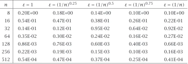
Table_6.5. _{Numerical results forExample 6.2(maximum error).}

n ε=1 ε=(1/n)0.25 _ε=(1/n)0.5 _ε=(1/n)0.75 _ε=(1/n)

8 0.20E+00 0.18E+00 0.14E+00 0.10E+00 0.10E+00

16 0.54E-01 0.47E-01 0.38E-01 0.26E-01 0.22E-01

32 0.14E-01 0.12E-01 0.95E-02 0.64E-02 0.92E-02

64 0.35E-02 0.30E-02 0.24E-02 0.16E-02 0.27E-02

128 0.86E-03 0.76E-03 0.60E-03 0.40E-03 0.66E-03

256 0.22E-03 0.19E-03 0.15E-03 0.10E-03 0.16E-03

512 0.54E-04 0.47E-04 0.37E-04 0.25E-04 0.41E-04

for differentnandε, whereν(x j)is the approximate solution of (1.1) obtained via (2.7) and (2.3).

Table 6.6 contains maximum errors based on the double-mesh principle (Doolan et al. [4]) (as forExample 6.3, the exact solution is not available):

max 0≤j≤nν

n

j−ν22jn, n=8,16,32,64,128,256. (6.9)

Tables6.3and6.7contain the numerical rate of uniform convergence for Ex-amples6.1and6.3, respectively, which is determined as in [4]:

rk,ε=log2

_z

k,ε zk+1,ε

, k=0,1,2, . . . , (6.10)

where

zk,ε=max j

ν_jh/2k−ν₂h/_j2k+1, k=0,1,2, . . . , (6.11)

Table_6.6. _{Numerical results forExample 6.3(maximum error).}

ε n=8 n=16 n=32 n=64 n=128 n=256 n=512

1/2 0.10E-01 0.25E-02 0.63E-03 0.16E-03 0.39E-04 0.98E-05 0.24E-05 1/4 0.20E-01 0.49E-02 0.12E-02 0.31E-03 0.77E-04 0.19E-04 0.48E-05 1/8 0.39E-01 0.96E-02 0.24E-02 0.60E-03 0.15E-03 0.38E-04 0.94E-05 1/16 0.75E-01 0.19E-01 0.47E-02 0.12E-02 0.29E-03 0.73E-04 0.18E-04 1/32 0.14E+00 0.35E-01 0.88E-02 0.22E-02 0.55E-03 0.14E-03 0.34E-04 1/64 0.25E+00 0.63E-01 0.16E-01 0.40E-02 0.99E-03 0.25E-03 0.62E-04 1/128 0.42E+00 0.11E+00 0.26E-01 0.66E-02 0.16E-02 0.41E-03 0.10E-03 1/256 0.64E+00 0.16E+00 0.40E-01 0.99E-02 0.25E-02 0.62E-03 0.15E-03

Table_6.7. _{Numerical results forExample 6.3(rate of convergence),}

n=8,16,32,64,128.

ε r (0) r (1) r (2) r (3) r (4) Avg

1/2 0.20E+01 0.20E+01 0.20E+01 0.20E+01 0.20E+01 0.20E+01 1/4 0.20E+01 0.20E+01 0.20E+01 0.20E+01 0.20E+01 0.20E+01 1/8 0.20E+01 0.20E+01 0.20E+01 0.20E+01 0.20E+01 0.20E+01 1/16 0.20E+01 0.20E+01 0.20E+01 0.20E+01 0.20E+01 0.20E+01 1/32 0.20E+01 0.20E+01 0.20E+01 0.20E+01 0.20E+01 0.20E+01 1/64 0.20E+01 0.20E+01 0.20E+01 0.20E+01 0.20E+01 0.20E+01 1/128 0.20E+01 0.20E+01 0.20E+01 0.20E+01 0.20E+01 0.20E+01 1/256 0.20E+01 0.20E+01 0.20E+01 0.20E+01 0.20E+01 0.20E+01

Table_6.8. _{Numerical results forExample 6.4(maximum error).}

ε Schatz’s: PL∗[9] Schatz’s: HC∗∗[9] Our results n=20 n=40 n=20 n=40 n=20 n=40

5−1 0.96E-03 0.24E-03 0.34E-05 0.26E-06 0.18E-14 0.60E-14 5−2 0.27E-01 0.60E-02 0.83E-03 0.90E-04 0.33E-15 0.56E-15 5−3 0.21E+00 0.12E+00 0.33E-01 0.94E-02 0.22E-15 0.22E-15 5−4 0.26E+00 0.26E+00 0.78E-01 0.68E-01 0.22E-15 0.22E-15 5−5 0.27E+00 0.27E+00 0.82E-01 0.82E-01 0.11E-15 0.11E-15 5−6 0.27E+00 0.27E+00 0.82E-01 0.82E-01 0.11E-15 0.11E-15 ∗_{PL: piecewise linears}

∗∗_{HC: Hermite cubics.}

1 0.8 0.6

0.4 0.2

0 0 0.1 0.2 0.3 0.4 0.5 0.6 0.7 0.8 0.9 1

Exact sol.

Approx. sol. forh=1/20

Figure_7.1. _{Exact and approximate solutions ofExample 6.1forε=} 0.001 without using fitting factor.

1 0.8 0.6

0.4 0.2

0 0 0.1 0.2 0.3 0.4 0.5 0.6 0.7 0.8 0.9 1

Exact sol.

Approx. sol. forh=1/20

Figure_7.2. _{Exact and approximate solutions ofExample 6.1forε=} 0.001 using fitting factor.

examples have been solved to demonstrate the applicability of the proposed method.

For Examples6.1and 6.3, we have computed the rate of convergence, see Tables6.3and6.7which show the uniform second-order convergence as pre-dicted in the theory. The same can be seen for the other examples also.

As is seen from Tables6.1and6.2, the results obtained using fitting factor are better than those without using fitting factor.

1 0.8 0.6

0.4 0.2

0 0 0.2 0.4 0.6 0.8 1

Exact sol.

Approx. sol. forh=1/20

Figure_7.3. _{Exact and approximate solutions ofExample 6.1forε=} 0.0005 without using fitting factor.

1 0.8 0.6

0.4 0.2

0 0 0.2 0.4 0.6 0.8 1

Exact sol.

Approx. sol. forh=1/20

Figure_7.4. _{Exact and approximate solutions ofExample 6.1forε=} 0.0005 using fitting factor.

Wahlbin [9] have solvedExample 6.4.Table 6.8shows (quite graphically) how badly standard methods can perform.

1 0.8 0.6

0.4 0.2

0 −1 −0.5 0 0.5 1 1.5 2

Exact sol.

Approx. sol. forh=1/40

Figure_7.5. _{Exact and approximate solutions ofExample 6.2forε=} 0.001 without using fitting factor.

1 0.8 0.6

0.4 0.2

0 −1 −0.5 0 0.5 1 1.5 2

Exact sol.

Approx. sol. forh=1/40

Figure7.6. Exact and approximate solutions ofExample 6.2forε= 0.001 using fitting factor.

are graphs without using fitting factor forExample 6.2forε=0.001 andε=

1 0.8 0.6

0.4 0.2

0 −2 −1.5 −1 −0.5 0 0.5 1 1.5 2

Exact sol.

Approx. sol. forh=1/40

Figure_7.7. _{Exact and approximate solutions ofExample 6.2forε=} 0.0001 without using fitting factor.

1 0.8 0.6

0.4 0.2

0 −1 −0.5 0 0.5 1 1.5 2

Exact sol.

Approx. sol. forh=1/40

Figure_7.8. _{Exact and approximate solutions ofExample 6.2forε=} 0.0001 using fitting factor.

Acknowledgement. The computations reported in this paper were done on Silicon Graphics Origin 200 (dual processor) Operating System (in Fortran 77 in double precision with 16 significant figures) at the Indian Institute of Technology Kanpur.

References

[1] J. H. Ahlberg, E. N. Nilson, and J. L. Walsh,The Theory of Splines and Their Ap-plications, Academic Press, New York, 1967.

[2] A. E. Berger, J. M. Solomon, M. Ciment, S. H. Leventhal, and B. C. Weinberg, Gener-alized OCI schemes for boundary layer problems, Math. Comp.35(1980), no. 151, 695–731.

[3] I. P. Boglaev,A variational difference scheme for a boundary value problem with a small parameter in the highest derivative, U.S.S.R. Comput. Math. and Math. Phys.21(1981), no. 4, 71–81.

[4] E. P. Doolan, J. J. H. Miller, and W. H. A. Schilders,Uniform Numerical Methods for Problems with Initial and Boundary Layers, Boole Press, Dublin, 1980. [5] J. J. H. Miller,On the convergence, uniformly inε, of difference schemes for a

two point boundary singular perturbation problem, Numerical Analysis of Singular Perturbation Problems (Proc. Conf., Math. Inst., Catholic Univ., Nijmegen, 1978), Academic Press, New York, 1979, pp. 467–474. [6] K. Niijima,On a three-point difference scheme for a singular perturbation problem

without a first derivative term. I, II, Mem. Numer. Math. (1980), no. 7, 1–27. [7] E. O’Riordan and M. Stynes, A uniformly accurate finite-element method for

a singularly perturbed one-dimensional reaction-diffusion problem, Math. Comp.47(1986), no. 176, 555–570.

[8] M. H. Protter and H. F. Weinberger,Maximum Principles in Differential Equations, Prentice-Hall, New Jersey, 1967.

[9] A. H. Schatz and L. B. Wahlbin,On the finite element method for singularly per-turbed reaction-diffusion problems in two and one dimensions, Math. Comp.

40(1983), no. 161, 47–89.

[10] J. M. Varah,A lower bound for the smallest singular value of a matrix, Linear Algebra and Appl.11(1975), 3–5.

[11] V. Vukoslavˇcevi´c and K. Surla,Finite element method for solving self-adjoint sin-gularly perturbed boundary value problems, Math. Montisnigri7(1996), 79–86.

Mohan K. Kadalbajoo: Department of Mathematics, Indian Institute of Technology, Kanpur-208016, India

E-mail address:[email protected]

Kailash C. Patidar: Department of Mathematics, Indian Institute of Technology, Kanpur-208016, India