ESTIMATION OF STRUCTURAL EQUATION MODELS THROUGH K MEANS CLUSTER APPROACH AN APPLICATION FOR ASSESSING SOCIO ECONOMIC DEVELOPMENT IN HARYANA

ESTIMATION OF STRUCTURAL EQUATION MODELS THROUGH

K- MEANS CLUSTER APPROACH - AN APPLICATION FOR

ASSESSING SOCIO - ECONOMIC DEVELOPMENT IN HARYANA

.

O.P. Sheoran, Lajpat Rai and K.K.Saxena* Department of Mathematics and Statistics

CCS Haryana Agricultural University, Hisar -125 004 (India)

*Department of Statistics, P.O.Box 338, UDOM, Tanzania

ABSTRACT

Structural equation models have been estimated with maximum likelihood technique

assuming three dimensions for socio-economic sectors. Scores for latent variables

from the best fitted model were computed by principal component analysis and

K-means cluster analysis. These models have been fitted for the purpose of studying

levels of socio economic development in Haryana State.

Keywords: Structural equation models, Maximum Likelihood Estimation, Cluster Analysis, Factor Analysis, Latent variables

Introduction

Socio-economic development in a region is related to the facilities of

education, transport, communication, electricity, financial institutions and medical

facilities etc. The pace of socio-economic development among various regions in a

State can never be uniform over the years owing to historic, geographic, ecological

and climatic conditions and some other unknown factors. Wide disparities may exist in

the level of development in different regions of the state.

The motivation to research workers has always been concerned to find out the

extent of these disparities with regard to agricultural, infrastructural, socio-economic

and industrial development parameters. Policy makers for the development of a State

need such systematic information to frame schemes, policies and programmes.

Statistically the problem is to identify the factors (latent variables) of

component analysis and k-means cluster analysis.

In the present paper, Principal component analysis has been employed to identify the

factors responsible for the development. Structural Equation Modelling (SEM) technique has

been used to develop the model of socio-economic development in the state of Haryana and

classify the tehsils according to their levels of socio-economic development. The assessment

of the overall fit of the model to data has been judged by Chi-square test statistic, Goodness

of fit index (GFI), Adjusted goodness of fit index (AGFI), Root mean square residual (RMR)

and Model modification Index.

Various authors have studied Multivariate techniques to distinguish regional

disparities for future planning in socio- economic aspects. Narain et al.(1991) used

multivariate technique for the first time to evaluate the economic development in Orissa .

Then in a series of papers, Narain et al. (1994,2001,2007 ,2012) studied the evaluation and

identification of development in various states of India. Lipshitz and Raveh,(1994,1998) used

the co-plot technique and Multi-dimentional scaling method for the socio economic

differences among various localities. Upadhyay (2001) used spatial and temporal analysis to

assess the development in Rajasthan. Soares et al., 2003, used factor and cluster analysis to

uncover regional disparities in the European Union. Sheoran et. al. (2012) estimated the

parameters of structural equation model with latent variables and used them for the

assessment of the development of Haryana State.

2. Methodology

The measurement model for each dimension in the form of standard factor analytical model is

given by

ε η Λ

y _y  (1)

for latent endogenous variables with E(εε)Θε and

δ

ξ

Λ

x



_x



(2)

for latent exogenous variables with E(δδ)Θ_δ

We also defineE(εδ)Θ_δεand E(ξξ)Φ, where

y is a p x 1 vector of observed indicators of the dependent (endogenous) latent variable

x is a q x 1 vector of observed indicators of the independent (exogenous) latent

variablesξ

η is a m x 1 random vector of latent dependent or endogenous variables

ξ is a n x 1 random vector of latent independent or exogenous variables

ε is a p x 1 vector of measurement error in y

δ is a q x 1 vector of measurement error in x

y

Λ is a p x m matrix of coefficients of regression of y onη and

x

Λ is a q x n matrix of coefficients of regression of x on ξ

The implied covariance/correlation matrix Σ(θ) is given by

δ x

xΦΛ Θ

Λ (θ

Σ )  

(3)

with the assumptions E(x) = E(δ) = 0 and E(ξδ’) = E(δξ’) = 0,

Then the structural part of the model is given by

ζ Γξ Βη

η   (4)

We also defineE(ζζ)Ψ, where

Β is a m x m coefficient matrix that relates endogenous variables to each other

Γ is a m x n coefficient matrix that relates endogenous variables to exogenous variables

and

ζ

is a m x 1 vector of errors (residuals)

The correlation matrix implied by the model is comprised of three separate correlation

matrices, i.e. correlation matrix of the observed indicators of the latent endogenous variables

yy

Σ ,the correlations between the indicators of latent endogenous and indicators of latent

exogenous variables isΣ_yxand the correlation matrix of the indicators of the latent exogenous

variablesΣ_xx.Arranging the above three matrices together, we get the joint covariance matrix

implied by the model, ie.















xx xy

yx yy

Σ

Σ

Σ

Σ

Σ(θ)

_.

                            _    δ x x δε 1 δε x 1 y ε y 1 1 y Θ Λ Φ Λ Θ Λ B) (I Γ Φ Λ Θ Λ ΓΦ B) (I Λ Θ Λ ] B) Ψ)[(I Γ (Γ B) (I Λ Σ(θ) y

x [ ]

(5)

After estimating an econometric model by maximum likelihood estimation procedure,

testing of the specific model (structural) formation, the latent scores for each of the modelled

latent variables for each unit (tehsil) were computed using the approach of Jöreskog (2000).

Consider the equations (1) and (2) for measurement models and writing these equations in a

system as given below





















































δ

ε

ξ

η

Λ

0

0

Λ

x

y

x y

and using the following notation

       x y Λ 0 0 Λ

Λ , _

      ξ η

ξa ,















δ

ε

δ

_a ,















x

y

x

_a ,

The latent scores for the latent variables in the model can be computed with formula

a 1 a UD VL VD UΛΘ x

ξ 2

1 2 1 2

1 _{ }

   

i

ˆ ₍₆₎

Where UDUis singular value decomposition of ΦE[ξ_aξ_a]and VLVis the value

of singular value decomposition of the matrix 2 1 2

1

UTBUVD

D , while Θ_ais the error

covariance/correlation matrix of the observed variables. The latent scores ξ_aiwere computed

for each observation xijin the [(pq)N] sample matrix whose rows are observations on

each of observed variables and N is number of tehsils. These latent scores (ξ_ai) were used as

an input for cluster analysis for the purpose of grouping the tehsils into several groups with

similar characteristics. At the first step, Ward (1963) hierarchical procedure has been used to

define the number of clusters and the group centroids. At second step, K-means method has

been applied by taking the centroids from the Ward (hierarchical) method as initial

seed-points. These steps were repeated until any re-assignment of cases does not make the clusters

more internally cohesive (homogeneous) and more clearly separated from each other.

For the purpose of developing structural equation models, we identified 9 indicators

for the year 2007-08, which have been included in the study. The codes and description of the

variables have been presented in Table 1.

Table1: Codes and description of the variables in socio-economic sector

Code Description Symbol

LITERACY Percentage literacy y1

LIT_MALE Male literacy rate y2

LIT_FEMALE Female literacy rate y3

BANK Average population per bank (in '000) y4

POP_DEN Density of population per square km of area x1

URBAN_POP Percentage of urban population x2

VEH_REG Different type of vehicles registered x3

M_WORKER Percentage of main workers to total population x4

COOP_SOC Number of co-operative societies per lakh of

population x5

The factor (latent variables) responsible for socio-economic development in the State

have been extracted by using Principal component analysis. The suitability of the factor

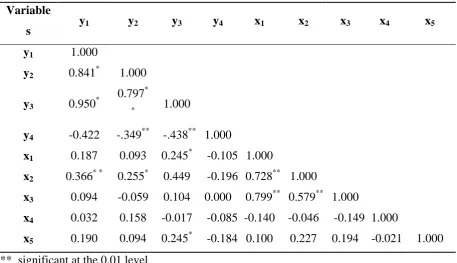
analysis has been tested by visual inspection of the correlation matrices (Table 2) , by the

Bartlett test of sphericity and by Keiser-Meyeer-Olkin (KMO) measure of sampling

adequacy. The Bartlett test produced the Chi-square values as 385.42 (P < 0.001) which

suggested that the original variables are significantly inter-correlated. The KMO statistic has

been obtained as 0.68 which suggests that there are sufficient numbers of indicators for each

factor. The Cattell’s scree plots (Fig 1) level out after third eigen value and the variance

contribution diminish after third component for all the periods, hence factor analysis has been

[image:6.595.137.449.81.296.2] [image:6.595.72.530.379.642.2]

Fig 1: Scree plot for the number of factors to be retained

Table 2: Correlation matrix of indicators variables for socio-economic sector.

Variable

s y1 y2 y3 y4 x1 x2 x3 x4 x5

y1 1.000

y2 0.841* 1.000

y3 0.950*

0.797*

* 1.000

y4 -0.422 -.349** -.438** 1.000

x1 0.187 0.093 0.245* -0.105 1.000

x2 0.366* * 0.255* 0.449 -0.196 0.728** 1.000

x3 0.094 -0.059 0.104 0.000 0.799** 0.579** 1.000

x4 0.032 0.158 -0.017 -0.085 -0.140 -0.046 -0.149 1.000

x5 0.190 0.094 0.245* -0.184 0.100 0.227 0.194 -0.021 1.000

** significant at the 0.01 level * significant at the 0.05 level

The normal varimax rotated solution for 9 selected indicators of socio-economic

sector have been given in Table 3. The Table 3 reveals that three components have eigen

values above one contributing 73.19 per cent of the total variance.

0.0 1.0 2.0 3.0 4.0

0 1 2 3 4 5 6 7 8 9 10

Ei

gen

Va

lue

The factor analysis suggested three factors have been found crucial for

socio-economic development. The first factor has significantly high loading on the variables

namely LITERACY, LIT_MALE, LIT_FEMALE and BANK. This factor could be taken as

dimension of “Literacy and Banking”. This factor explains 38.73 per cent of the total

variance. The second factor has been identified as “Population Distribution and Vehicles” as

it loads very heavily on the variables like POP_DEN, URBAN_POP and VEH_REG. This

factor explains 23.69 per cent of the total variance. The third factor “Work Force” loads high

on M_WORKER only. This factor explained 10.76 per cent of the total variance.

A perusal of communality values indicates that for 7 variables, the communalities

exceed 70 per cent. Thus there is a fair degree of representation of all the 9 considered

variables by the three factors i.e. “Literacy and Banking”, “Population distribution and

vehicles” and “Work Force” identified crucial for socio-economic development.

In order to normalize these variables using monotonic transformation technique ,

these variables have been transformed to Normal distribution by normal score technique

(Jöreskoget al. 2000).

Table3: Normal varimax solution for variables of socio-economic Sector

Variables Factor 1 Factor 2 Factor 3 h2

LITERACY _{0.95 0.13 -0.04 0.92} LIT_MALE _{0.90 -0.01 0.10 0.81} LIT_FEMALE _{0.94 0.19 -0.09 0.93} BANK _{-0.57 -0.07 -0.15 0.35} POP_DEN _{0.07 0.93 -0.05 0.87} URBAN_POP _{0.31 0.81 0.02 0.77} VEH_REG _{-0.08 0.91 -0.08 0.83} M_WORKER _{0.07 -0.09 0.98 0.98} COOP_SOC _{0.24 0.25 -0.05 0.13}

Eigen Value _{3.49 2.13 1.17}

Percentage variance _{38.73 23.69 10.77} Cumulative

The structural equation model of socio-economic sector of Haryana has been

hypothesized on the basis of the three latent variables as suggested by the preliminary

exploratory factor analysis and then further improved by freeing the elements of residual

matrices and adding or deleting the indicator variables to the latent variables as suggested by

the largest modification indices. The model parameters have been re-estimated after every

improvement. Finally, the model which converged to the optimum solution with acceptable

fit statistics has been obtained. The exogenous measurement models using (2) of socio

-economic sector have been given in matrix equation (7) as given below:

                                                        5 4 3 2 1 2 1 ) ( 52 ) ( 41 ) ( 32 ) ( 31 ) ( 22 ) ( 11 5 4 3 2 1 0 0 0 0              x x x x x x x x x x x (7)

From the equations (7), it can be revealed that the exogenous latent variable ξ1 has

been measured by POP_DEN, VEH_REG with positive factor loadings and M_WORKER

with negative non-significant loading. The second latent dimension ξ2has positive significant

loadings on indicator variables like URBAN_POP, VEH_REG and COOP_SOC.The

endogenous measurement model using (2), has been formulated as

 

                                        4 3 2 1 1 ) ( 41 ) ( 31 ) ( 21 ) ( 11 4 3 2 1          y y y y y y y y (8)

The endogenous measurement model presented in (10) depict that the latent variable

η1 has been measured by the indicator variables namely LITERACY,LIT_MALE,

LIT_FEMALE and BANK.The structural equation model with latent variables using (3), has

been given by following equation

1 2 12 1 11

1













   (9)

The restricted model has been estimated by setting the off-diagonal elements of _

and _ to zero. The restricted model has a Chi-square value of 30.90 (d.f = 24) with GFI =

0.90 and SRMR = 0.07 showing that it does not fit well to the data. The restricted models

matrices. The residual matrix of endogenous variables remained as diagonal matrix as given

below in (10).

                         44 33 22 11 0 0 0 0 0 0 (10)

In order to obtain the improved model which fit well to the data, certain elements of

Θδ and Θδϵ have been kept free as given below in (11) and (12).The improved model has

Chi-square value as 3.91 (d.f.=15), GFI as 0.99 and SRMR as 0.03 showing that model implied

correlation matrix is equal to population correlation matrix.

                               55 44 33 22 21 11 0 0 0 0 0 0 0 0 0 (11) and                   0 0 0 0 0 0 0 0 0 0 0 0 52 51 43 42 32 23 13 12                  (12)

The path diagram of final models which fit well to data for socio-economic sector

[image:9.595.117.482.553.722.2]

with estimated coefficients has been presented in Fig 2.

Table4: Maximum likelihood estimates of structural equation model for socio-economic

sector

Parameter Estimate (S.E) Standardize

d Estimates Parameter Estimate (S.E)

Standardized Estimates

) ( 11

x

 0.91 (0.16) 0.92 ₄₄ 0.94 (0.17) 0.94

) ( 22

x

 0.57 (0.16) 0.57 55 0.78 (0.18) 0.79 )

( 31

x

 0.68 (0.15) 0.68 ₂₁ 0.17 (0.10) 0.18

) ( 41

x

 -0.25 (0.13) -0.25 ₁₁ 0.04 (0.03) 0.04

) ( 52

x

 0.46 (0.17) 0.46 ₂₂ 0.28 (0.05) 0.29

) ( 11

y

 1.00 0.98 33 0.11 (0.03) 0.11 )

( 21

y

 0.86 (0.07) 0.84 ₄₄ 0.79 (0.14) 0.79

) ( 31

y

 0.97 (0.05) 0.94 ₁₂ -0.12 (0.06) -0.12

) ( 41

y

 -0.46 (0.11) -0.45 13 0.06 (0.04) 0.06

21



0.46 (0.19) 0.46 23 0.14 (0.05) 0.14

11



0.05 (0.21) 0.05 32 -0.15 (0.07) -0.15

12



0.64 (0.24) 0.66 ₄₂ 0.14 (0.07) 0.14 var(ζ1) 0.51 (0.21) 0.53



₄₃ -0.07 (0.04) -0.07



₁₁ 0.14 (0.24) 0.15 51 -0.08 (0.05) -0.08



22 0.67 (0.17) 0.68



52 -0.20 (0.07) -0.20



33 0.53 (0.16) 0.53

χ2

(df=15) 3.91

GFI 0.99

SRMR 0.03

The un-standardized and standardized maximum likelihood estimates of the free

parameters of models have been presented in Table 4. The estimates in Table 4 indicated that

the exogenous variable ξ1 has a positive non-significant influence on the endogenous latent

variable η1 whereas exogenous latent variables ξ2 indicates a positive significant influence on

η1. Also the exogenous latent variables ξ1 and ξ2 have significant correlation. The estimates in

the Table 4 also revealed that the off-diagonal elements ₂₁ of the residual matrix _have

Using (6), the latent scores ξ_aiwere computed for each observation xij in the

] )

[(pq N sample matrix whose rows are observations on each of observed variables and

N is number of tehsils.These latent scores (ξ_ai) were used for classifying the tehsils with

cluster analysis. In order to search for the number of groups which shows similar

socio-economic characteristics, Ward’s hierarchical clustering method has been used on the latent

scores of three socio-economic dimensions. The Ward’s method based on squared Euclidean

distances has been used to form the dendogram (Fig 3). From the analysis the dendogram, it

has been concluded that 3-clusters solutions are appropriate for grouping of tehsils on the

basis of socio-economic characteristics. The average scores on the latent variables η1, ξ1 and

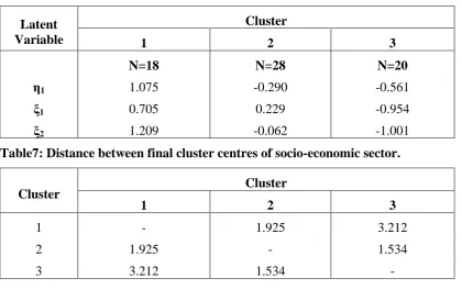
[image:11.595.71.525.304.660.2]

ξ2 for the resulting three clusters are presented in Table 5.

Fig 3: Dendogram for socio-economic sector

Table5: Cluster centroids

Cluster η1 ξ1 ξ2

1 1.209 -0.179 -0.742

2 0.682 0.223 -1.127

B alabg arh Na ra ing arh Ishar ana P anc hkula B ara ra R ewa ri F arida ba d Gur g aon Amba la

Nuh _Firoz

pur Jhirka Ja g adha ri

Hisar Sohna Jha

jhar

P

anipat _Karna

l

P

ataudi

S

onipat _Baha

durg arh Gha ra unda P ehowa Ga na ur Nilokher i S afidon Ka laka B hiwa ni Maha m Julana Ellena ba d B awa ni Khe ra S hiwa ni L oha ru Na rna und Ada mpur C h. Da dr i B awa l Kha rkhod a Hoda l Toha na R ati a F eteha ba d Tosha m R ania

Guhla Kosli Assa

nd S irsa Da bwa li B eri C hha chhra uli Ha nsi S ha hba d S amala kha Ka it ha l Tha ne sa r P nha na P alwa l R ohtak Ta vr u

Jind _Narna

3 1.340 -0.129 -0.975

The non-hierarchical clustering procedure (K-means), using the cluster centres

presented in Table 5 of hierarchical solution as the initial seed points has then been used to

improve the results of best cluster solution derived by the Ward’s method. The improved

cluster solutions by K-mean procedure for the socio-economic sector have been presented in

Table 6. The perusal of the Table 6 indicated that cluster 1 comprising of 18 tehsils as

mentioned in Table 8 has been characterised by high scores on all the latent variables. The

Cluster 2 has moderately higher scores on all the latent variables compared to cluster 3 and

consisting of 28 tehsils as mentioned in Table 8. The remaining 20 tehsils form cluster 3

which has lower scores on all the latent dimensions. The largest distance of 3.212 between

the cluster 1 and 3 has also supported this fact that these clusters differ significantly with

respect to socio-economic characteristics. Further, the distance between cluster 1 and 2 as

well as cluster 2 and 3 indicates that these clusters are also dissimilar in socio-economic

characteristics.

Table6 : Final cluster centres of socio-economic sector

Latent Variable

Cluster

1 2 3

N=18 N=28 N=20

η1 1.075 -0.290 -0.561

ξ1 0.705 0.229 -0.954

[image:12.595.72.493.405.668.2]

ξ2 1.209 -0.062 -1.001

Table7: Distance between final cluster centres of socio-economic sector.

Cluster Cluster

1 2 3

1 - 1.925 3.212

2 1.925 - 1.534

Table8 : Classification of tehsils for socio-economic development in Haryana State.

Cluster Tehsils

1 Hisar, Panchkula, Asandh, Isharana, Gurgaon, Sohna, Nuh, FirozpurJhirka, Faridabad, Balabgarh, Jagadhari, Kaithal, Sirsa,

Ambala, Barara, Narayangarh, Jhajhar, Rewari

2

Adampur, Hansi, Narnaund, Gohana, Fatehabad, Ratia, Narnaul,

Mahendergarh, Indri, Smalakha, Taoru, Punhana, Palwal, Rohtak,

Chhachhrauli, Jind, Narwana, Guhla, Thanesar, Shahbad, Dabwali,

Rania, Tosham, Siwani, Loharu, CharkhiDadri, Beri, Kosli

3 Sonipat, Kharkhoda, Ganaur, Tohana, Kalaka, Karnal, Gharaunda, Nilokheri, Panipat, Pataudi, Hodal, Meham, Julana, Safidon, Pehowa,

Ellenabad, BawaniKhera, Bhiwani, Bahadurgarh, Bawal

References

Joreskog, K.G. (2000). Latent variable scores and their uses. Scientific Software International, http://www.ssicentral.com/lisrel.

Joreskog, K.G., D. Sorbom, S.duToit and M. du Toit (2000).LISREL 8: New Statistical Features. Chicago: Scientific Software International.

Lipshitz, G. and A. Raveh (1994). Application the Co-Plot Method in the Study of Socio-economic differences among Cities: A Basis for a Differential Development Policy.

Urban Studies, 31: 123-135.

Lipshitz, G. and A. Raveh (1998). Socio-economic differences among localities: A new method of multivariate analysis. Regional Studies, 32: 747–757.

Narain, P., S.C. Rai, and P. Sarup (1991).Statistical evaluation of development on socio-economic front.Jour. Ind. Soc. Agric. Stat.43(3): 329-345.

Narain, P., S.D. Sharma, S.C. Rai and V.K. Bhatia (2001).Regional dimensions of disparities in crop productivity in Uttar Pradesh.Jour. Ind. Soc. Agric. Stat.54: 62-79.

Narain, P., S.D. Sharma, S.C. Rai and V.K. Bhatia (2007).Statistical evaluation of social development at district level.Jour. Ind. Soc. Agric. Stat.61(2): 216-226.

Soares, J.O.; M.M.L Marqus and C.M.F. Monteiro.(2003). A multivariate methodology to uncover regional disparities: A contribution to improve European Union and governmental decisions. European Journal of Operational Research, 145: 121–135.

Upadhyay, B. 2001.Statistical Assessment of Development in Rajasthan – A Spatial and Temporal Analysis. Unpublished Ph.D. Thesis, M.P.U.A.T, Udaipur.