Volume 2012, Article ID 515192,20pages doi:10.1155/2012/515192
Research Article
Maximum Likelihood Estimators for a Supercritical
Branching Diffusion Process
Pablo Olivares
1and Janko Hernandez
21Department of Mathematics, Ryerson University, Toronto, ON, Canada M5B 2K3
2School of Business, ITAM, 01000 Mexico City, DF, Mexico
Correspondence should be addressed to Pablo Olivares,[email protected]
Received 29 June 2012; Accepted 18 October 2012
Academic Editor: Angelo Plastino
Copyrightq2012 P. Olivares and J. Hernandez. This is an open access article distributed under
the Creative Commons Attribution License, which permits unrestricted use, distribution, and reproduction in any medium, provided the original work is properly cited.
The log-likelihood of a nonhomogeneous Branching Diffusion Process under several conditions
assuring existence and uniqueness of the diffusion part and nonexplosion of the branching process.
Expressions for different Fisher information measures are provided. Using the semimartingale
structure of the process and its local characteristics, a Girsanov-type result is applied. Finally, an Ornstein-Uhlenbeck process with finite reproduction mean is studied. Simulation results are discussed showing consistency and asymptotic normality.
1. Introduction
Some spatial-temporal models are often used to describe the behavior of particles, which are moving randomly in a domain and reproducing after a random time.
We consider a Branching Diffusion ProcessBDP, consisting in particles performing independent diffusion movements and having a random numbers of children at random times.
In1, for example, a simple model of cells with binary splitting after an exponentially distributed random lifetime is considered, where cells move according independent Brownian motions.
In5, a particle system is considered in a more general context, where interaction among individuals is allowed. There, a link between the associated martingale problem and the infinitesimal generator is established. For a noninteracting BDP, the uniqueness of the martingale problem is found in 6 together with the analysis of the limit behavior of the process.
On the other hand, the statistical approach of this kind of models remains less explored. In 1, under continuous observations upon a fixed time T, it obtained the maximum likelihood estimators for the variance and the rate of death of a Brownian motion with a deterministic binary reproduction law. In 7, using a least square approach the parameters of the BDP are also estimated.
In8,9, a birth and death processes in a flow particle system are considered. There, the absolute continuity of the probability law for the corresponding canonical process is obtained. We follow a similar approach, but allowing the possibility to have more than one particle at birth times, as our case, in which introduces additional complexity due to the exponential growth of the model.
There are many inference results for branching processes as well as for the diffusion process separately; we essentially consider both aspects together via a measure-valued process describing the particle configuration at any time. The functions describing the model
i.e., drift, death rate, and reproduction lawdepend on a common unknown parameter. As in the model mentioned above, technical difficulties arise in writing the corresponding likelihood function. We use a Girsanov theorem for semimartingales, as given, for example, in 10, allowing the passage from a BDP reference measure to another one depending on the true value of the parameter. The semi-martingale structure of the process and its corresponding local characteristics under the change of measure are obtained using ˆIto’s formula.
The covariance matrix of the diffusion part is assumed to be known in order to avoid singularity with respect to the reference measure; otherwise the quadratic variation can be used as a nonparametric estimator of the former.
Expressions for the observed and expected Fisher information measures are provided. In a companion paper, see 11, the asymptotic behavior of these measures is studied, and consequently, the consistency and asymptotic normality of the maximum likelihood estimators.
The organization of the paper is as follows.
InSection 2, we establish the model and the main notations. Also, we give certain
sufficient conditions in order to have the existence of diffusion model and the nonexplosion on finite time of the branching part. These conditions are standards in both types of models.
InSection 3, we obtain the semi-martingale structure of the model from ˆIto’s formula and
we calculate the local characteristics of the BDP. InSection 4, we find the likelihood function of the model using a Girsanov-type theorem for semi-martingales. Finally, inSection 5we present an example, the Branching Ornstein-Uhlenbeck process, where explicit estimators can be obtained.
2. Model and Main Notations
We establish the main features of our model.
certain random time, depending on its trajectory. At the time of its death, it gives birth to an also random number of particles which continue to move from the ancestor position and reproduce in the same way.
Let U be the set of all particles that can appear in the system; we represent U by ∞
n1Nn.
With every particleu∈ Uwe associate a random vectorsu, τu, Nu,Xu
tt∈R wheresu
andτuare its birth and the death times, respectively, taking values on0,∞,Xu
t is its position at timet, andNurepresents the number of offsprings.
At the initial timet0, we have a configuration given by a finite number of particles denoted byu1, u2, . . . , uN ∈ Uat respective deterministic positionsx1, x2, . . . , xN. According to notations we establish
su1su2· · ·suN 0, Xu1
0 x1, X
u2
0 x2, . . . , X
uN
0 xN. 2.1
We define recursively the random variablessu,τu, andXu
t in the following way.
Suppose a particlevdies, giving birth to a particleuamong its descendants; we set
su τv. At timesu, the particleumoves according to a diffusion process with driftb·and infinitesimal varianceσ·then
Xu t Xsuu
t
0
1su,∞sbXsuds
t
0
1su,∞sσXsu·dWsu fort≥0, 2.2
whereWu Wu
tt∈R is a standard Brownian motion inRd.
The death rateλ·function, for a particle located atxat timet, satisfies
Prτu≥t Δt|τu ≥t≥su; Xut x
λxΔt oΔt. 2.3
Finally, the probability law representing the reproduction law of a particle located at pointx, and denoted bypkxk∈N,x∈Rdverifies
PrNuk|Xuτu x pkx. 2.4
ProcessesWu
u∈UandNvv∈Uare independent.
We describe the process of living particles by the measure-valued processM Mtt≥0,
where
Mt
u∈U
1su,τutδXu
t. 2.5
Hereδxdenotes the Dirac measure onRd,BRd, whereBRdis the Borelianσ-algebra in Rd.
Notice that for A ∈ BRd,M
The processMis a Markov process called Branching Diffusion Process. For existence and properties see, for example,5. This process takes values in
E
n
i1
δxi :n0,1,2, . . .; xi∈Rd
2.6
a closed subspace ofMFRd, the space of finite Borel positive measures onRd.
Denote byCbRdthe set of bounded and continuous functions onRd. For everyf ∈
CbRd, we define the normfsup{|fx|:x∈Rd}.
For everyξ∈MFRdandf:Rd → R, measurable we set
ξ f
Rd
fdξ. 2.7
We will note for X, Y and X, Y the covariance process and the quadratic covariance process. AlsoXpis the projection ofXin the sense described in10.
We introduce the following spaces:
V: class of right continuous-adapted processes with left limits and with finite variations on finite intervals starting at the origin at time 0;
V : class of processes inVwith nondecreasing trajectories;
A: class of processes in V with EVarA∞ ≤ ∞, where VarA is the variation process associated toA;
A : class of processes inVwithEA∞≤ ∞; MP: class of uniformly integrable martingales.
AlsoVloc,Vloc,Aloc,Aloc, andMPlocare the corresponding local classes.
We takeMtt∈R as the canonical process in the stochastic basisΩ,F,F, Pm, where
mis a given initial configuration, following its usual construction.
By assuming that the functions driving the model depend on an unknown parameter
θ, a statistical model associate to the process is considered.
More specifically letΘ ⊂Rm be an open and convex set representing the parametric space and assume thatb,λ, andpdepend on a parameterθ∈Θ, then we have
b:Θ×Rd−→Rd bθ;x bθx bθix
i1,...,d,
σ:Rd−→Rd⊗Rd σx σ
ijx
i,j1,...,d,
λ:Θ×Rd−→R∗ λθ;x λθx,
p:Θ×N×Rd −→0,1 pθ;k, x pkθ;x pkθx.
2.8
HereRd⊗Rdis the space ofd×dreal-valued matrices. When no confusion is possible we will note by| · |a norm in the spaceRd⊗Rdas well as the Euclidean norm inRd. These functions define, for a given initial configurationmand any parameterθ, a probabilityPθ
Suppose now these functions satisfy the following properties for everyθ∈Θ.
A1 Lipshitz Local Condition. For alln≥1, there exists a constantCθ
n>0 such that
bθx−bθ y σx−σ y≤Cθnx−y ∀|x| ≤n, y≤n. 2.9
A2 Linear Growth Condition. There exists a constantK >0 nondepending onθsuch that
bθx |σx| ≤K1 |x| ∀x∈Rd. 2.10
A3σxis an invertible matrix for allx∈Rd, hence
ax σxtσx 2.11
is symmetric and positive definite.
A4For allx∈Rdwe have
∞
k0
pkθx 1. 2.12
A5Let
mθx
∞
k0
kpθkx,
κθx
∞
k0
k−12pθkx
2.13
thenλθ,mθ, andκθbelong toC
bRdwith
λθx≤λθ, mθx≤mθ, κθx≤κθ ∀x∈Rd. 2.14
A6There exist constantsλθ
o>0 andmθo>1 such that
λθx≥λθo, mθx≥mθo>1 ∀x∈Rd. 2.15
Remark 2.1. A1andA2are standard conditions in order for the existence and uniqueness
of the stochastic differential equations describing particle diffusions.
Remark 2.2. The infinitesimal covariance does not depend onθ. In general, we cannot have
Remark 2.3. The second part ofA6is a uniform supercritical condition necessary to avoid the almost sure extinction of the branching process.
Let’s now define
γθ inf
x∈Rdλ
θxmθx−1, γθsup
x∈Rd
λθxmθx−1. 2.16
FromA5andA6we have
γθ≤λθmθ−1,
γθ≥λθo
mθo−1
2.17
then
0< γθ≤λθxmθx−1≤γθ<∞ ∀x∈Rd. 2.18
The expression λθxmθx−1 is the generalized Malthus parameter, see, for example,
12,13.
We assume that the whole process is observed on an interval0, T; that is, at every time we observe the entire configuration of particles.
We need to deal with the jumps of the process; to this end we define
ΔMtMt−Mt−, 2.19
whereMt−is the left limit of processMtt≥0at timet.
Let’s denote by 0< T1< T2<· · ·< Tn<· · · the times at which the jumps of the process take place, then, if at timeTna particle dies at positionXnand hasKnoffsprings we have
ΔMTn KnδXn−δXn. 2.20
The space of jumps is a closed subset ofMFRddefines as
Sdk−1δx:k∈N, x∈Rd
. 2.21
Let alsoμMbe the random measure associated with the jumps ofMgiven by
μMdt, dx
s≤t
Finally, for every optional functionWonR ×Sdand a random measureνonBR ×Sdwe define the processW∗νby
W∗νt t
0
Sd−{0}
Ws, xνds, dx. 2.23
3. Martingale Representation of the Process and Local Characteristics
We study now the local characteristics of the processMthrough the real processMf
Mtft≥0.
The following result gives its semi-martingale structure, a useful decomposition of the process in a bounded variation process, a continuous martingale, and a purely discontinuous martingale.
Theorem 3.1. For every functionf:Rd → RinC2Rd, the processMfis decomposed as
Mt f
M0 f
t
0
Ms
Aθfds Rft idf ∗μMt, 3.1
where
Rft
u∈U t
0
1su,τus tDf·σXus·dWsθ,u 3.2
is a square integrable martingale with zero mean underΩ,F,F, Pθ
mand
Aθfx 1
2 d
i,j1
aijxDi,jfx d
i1
bθixDifx 3.3
is the infinitesimal generator of the common diffusion law followed by the particles andidf :t,k−
1δx→k−1fxis optional onR ×Sd.
HereDiandDi,jrepresent the first derivative with respect toxiand the mixed second derivative
with respect toxiandxj, respectively, whereasD=tD1, D2, . . . , Dd.
Proof. We apply ˆIto’s formula to process2.2forf∈C2Rd. Then we replace t byτu∧tand
we get
f Xu
τu∧t
−fXu
su
t
0
1su,τusAθfXsuds
t
0
Adding3.4for everyu∈ U, the right hand side is
t
0
u∈U
1su,τusAθfXsu
ds
u∈U t
0
1su,τustDf·σXus·dWsu
t
0
Ms Af
ds Rft.
3.5
On the other hand, the left hand side can be written as
u∈U:su≤t
f Xτuu∧t
−fXusu
u∈U:su≤t<τu
f Xtu
u∈U:τu≤t
fXτuu−
u∈U:su≤t
fXusu
Mft−Mf0−
0<s≤t
ΔMfs
Mft−Mf0−idf ∗μMt.
3.6
By definitionidf ∗μM−νθis a local martingale, whereνθis the compensator of the processMthen by adding and subtractingidf∗νθwe have the following.
Corollary 3.2. For everyf ∈C2Rdthe process
Mt f
−M0 f
−
t
0
Ms
A∗,θfds 3.7
is, under Ω,F,F, Pθ
m, a square integrable local martingale with zero mean and quadratic
characteristic:
t
0
Ms
tDf·a·Df λθκθf2ds. 3.8
Here,
A∗,θfAθf λθmθ−1f. 3.9
Proposition 3.3. LetXbe a real-adapted process, h a truncating function,A∈ Vcontinuous,C∈ V
continuous, andνa random measure inR ×Rdsuch thatνdt, dy K
tdydt. LetBA h∗ν.
ThenXis a semimartingale with local characteristicsB, C, νwith respect to a truncating function
hif and only if for everyF ∈C2Rthe process
FXt−FX0−
t
0
FXs−dAs−1 2
t
0
FXs−dCs−
F Xs− y−FXs−∗νt 3.10
is a local martingale.
Proof. It is enough to see thatB∈ Vis a continuous process and
t
0
FXs−dh∗νs t
0
FXs−
Rh y
Ks dy
ds
0,t×RFXs−h y
ν ds, dyFXs−h y∗νt.
3.11
Also,
y2∧1∗νt t
0
R
y2∧1Ks dy
ds
t
0
Hsds, 3.12
whereHis a nonnegative process theny2∧1∗ν∈ V . Moreover, it is continuous therefore
predictable and it belongs toAloc⊂ Aloc.
We have the following result.
Theorem 3.4. For anyθ∈Θandm∈Edthere exist a probabilityPθ
mon as stochastic basisΩ,F,F
such thatΩ,H,H, Pθ,m. We haveM0 ma.s. andBf, Cf, νfwhich are the local characteristics
ofMfwith respect tohfor anyf∈C2bRd. The restrictionP
θ,mtoFis the only probability in the
filtered spaceΩ,F,Fwith these local characteristics. HereBf, Cf, νfare given, for any truncating
functionhby
Bft
t
0
Ms−
Aθf·ds h∗νft,
Cft
t
0
Ms−,t Df·a·Df·
ds
3.13
andνf onR ×Rdas
νf dt, dyM
t−
λ·
∞
k0
pθ
k·δk−1f· dy
or equivalently, for every optional functionwonR ×Rd:
w∗νft
t
0
Ms−
λ·
∞
k0
pk·w s,k−1f·
ds. 3.15
Proof. From5, Theorem 3.1, or6, Chapter 5, we have the existence of a probability measure
inΩ,F,Fmaking2.5a BDP with infinitesimal generatorGθAθ Bθwhere
AθF μ fF μ fμAθf 1 2F
μ fμ tDfaDf,
BθF μ fμ
λθ·
∞
k0
pθk·F μ f k−1δ. f
−F μ f
.
3.16
Moreover, for every non negative functionF∈C2bRandf∈C2bRdwe have that
F Mt f
−F m f−
t
0
GθF M
s−fds 3.17
is a local martingale with respect toΩ,F,F, Pθ m. We can write3.17as
F Mt f
−F M0 f
−
t
0
F Ms− fMs−
Aθfds−1
2 t
0
FMs−Ms− tDf ·a·Dfds
− t
0
Ms−
λθ∞ k0
pθ k
FfMs− k−1δ.−FfMs−
ds
F Mtf
−F M0f
−
t
0
F Ms−fd s
0
Mr−
Aθfdr
−1 2
t
0
F Ms−fd s
0
Mr− tDf·a·Dfdr
−F Ms−f y−F Ms−f∗νf ds, dyt.
3.18
From the last expression we apply the precedent proposition and identify the local characteristics as those in expressions3.13and3.15.
4. Absolutely Continuous Measure Changes, Likelihood Function,
and Fisher Information Measures
As reference measure we take the one determined by
b0x 0,
λ0x 1,
p0kx 1
2k 1,
4.1
that is, particles moving according to independent Brownian motions without drifts. In the sequel, as we start from a fix deterministic configuration M0 m, we will drop the
dependence onm, then we denote byP0andPθthe respective probabilities generated by the reference measure and the functions given in2.8according toTheorem 3.4. We will denote byE0andEθthe expectations underP0andPθ, respectively.
It is well known that the semi-martingale structure persists after an absolutely continuous change of the probability measure. In order to see how the local characteristics change with it we construct a probability measureQθ, absolutely continuous with respect to
P0, with the same local characteristics thanPθ, thereforeQθandPθare a.s. equal. LetB0, C0, ν0be the local characteristics of the process underP0given by
B0ft t
0
Ms− A0f
ds hf ∗ν0
t,
C0ft t
0
Ms− tDfaDfds,
W∗ν0t t
0
Ms−
λ0·
∞
k0
p0k·Ws,k−1δ.
ds,
4.2
where
A0fx 1
2 d
i,j1
Dijfxaijx. 4.3
Equations3.13and3.15can be, respectively, rewritten as
Bft
t
0
Ms−
Aθfds hf∗νt,
CftC0,
W∗νt
t
0
Ms−
λθ
∞
k0
pθkWs,k−1δ.
ds,
4.4
where
Aθf A0f tDf·b. 4.5
Next, we define the functiony:Sd → R as
yk−1δx
λxpθkx λ0xp0
kx
4.6
wheneverλ0xp0
kx/0 and zero are otherwise.
Also we define the following processes onΩ,F,F:
Yt
u∈U t
0
1su,τu
tb·a−1Xu
s·dXus y−1
∗μM−ν0
t, 4.7
Ztexp
Yt−1 2Y
c t
0<s≤t
1 ΔYse−ΔYs. 4.8
Note thatY is well defined on the basisΩ,F,F, P0. Indeed,
y−1∗ν0 t
t
0
Ms−
λ0
∞
k0
p0λ
θpθ k
λ0p0
k −1 ds ≤ t 0
Ms−
λ0
∞
k0
λθpθ k
λ0 p
0 k ds t 0
Ms−
λ0 λθds≤λ0 λθ
t
0
Ms1ds
4.9
then|y−1| ∗ν0∈ AlocP0and it is predictable.
Moreover,
E0 y−1∗ν0
t
≤λ0 λE
t
0
Ms1ds
<∞. 4.10
Theny−1∗μM−ν0is a purely discontinuous local martingale onΩ,F,F, P0.
The first term in Y is a local continuous martingale so the process Y is a local martingale. Their jumps have the form
ΔYt1ΔMt/0 yΔMt−1
4.11
then
1 ΔYt
1 if ΔMt0,
yΔMt if ΔMt/0.
4.12
Let Rnn∈N be now a sequence of local stopping times forZ; we note by P0,Rn the
restriction ofP0to theσ-algebraFRn and we define on it the probability measureQnasdQn
ZRndP
0,Rn, whereZRnis the processZstopped at timeTn.
We have the following result.
Proposition 4.1. The local characteristics ofQnare given by3.13and3.15.
Proof. Let’s note byBn, Cn, νnthe local characteristics ofMunder the measureQ
n. First, note that ifWinR ×Sdis an optional process then
W∗ yν0
tωt Wy∗ν0
tωt
t
0
Ms−
λ0
∞
k0
p0kWs,k−1δ.
λθpθ k
λ0p0
k
ds
t
0
Ms−
λθ
∞
k0
pθkWs,k−1δ.
dsW∗νt,
4.13
hencedνydν0and in a similar way we havedνRn ydν0Rn.
On the other hand,
Ztexp
Yt−−12Yct
0<s<t
1 ΔYse−ΔYs
1 ΔYt 4.14
thenZZ−1 ΔYand
1ΔMRn
t /0Z
Rn
t 1ΔMRnt /0ZtR−ny
ΔMRn
t
. 4.15
Thus, we have that for everyP ⊗ S-measurable functionU:Ω×R ×S → Rd,
t
1ΔMt/0ZtUt,ΔMt
t
1ΔMt/0yΔMtZt−Ut,ΔMt 4.16
or equivalently
ZU∗μX∞yZ−U∗μX∞. 4.17
Hence,
EZU∗μX
∞
EyZ−U∗μX∞
. 4.18
According to10, Theorem III.3.17,yZ−is a version of the conditional expectationMPμMZ|
P ⊗ Sand consequentlyyν0is a version of the compensator ofμXon the basisΩ,F,F, Qθ.
Then we haveνnν.
Next, we defineNRf hf∗μM−ν0andNn N−N, YpRn, whereNRn is the
We can see thatNn∈ M
locQn. Indeed,NRn ∈ MlocP0and its jumps
ΔNRn 1
ΔMf/0hf ΔMf
≤ h 4.19
are bounded; hence combining Theorem III.3.11, Lemma III.3.14 in10we have that
Nn N−N, YpRn ∈ M
locQn. 4.20
Moreover,
N, Y Rf, Yc
0<s≤t
ΔNsΔYs
Rf, Yc h
f y−1
∗μM
4.21
and then
N−N, YpRf hf∗
μM−ν0
−Rf, Yc−hf∗ν hf∗ν0
Rf−Rf, Yc hf∗
μM−ν.
4.22
We can write
Nn Rf−Rf, YcRn
hf∗
μM−νRn ∈ MlocQn. 4.23
As
hf ∗
μM−νRn hf∗
μMRn −νRn
∈ MlocQn 4.24
we have
Rf−Rf, YcRn ∈ M
locQn. 4.25
From3.1,
MRn
t fMR0nf
t
0
Ms A0f
ds Rf
Rn
id∗μMt Rnf
MRnf 0
t
0
Ms A0f
ds Rf, Yc
Rn
Rf−Rf, YcRn
id∗μMt Rnf
with
Rf, Yc
u∈U t
0
1su,τustDf·σXus·dWsu,
u∈U t
0
1su,∞st
σ−1·bθXu s·dWsu
t 0 Ms
tDf ·bθds.
4.27
We identifyBnandCnas3.13usingProposition 3.3.
From the previous proposition we get the following.
Theorem 4.2. Under conditions (A1)–(A6) in the spaceΩ,F,Fwe have for anyθ∈ΘthatPθ
loc
P0with densityZgiven by4.8.
The log-likelihood is given by
ltθ
u∈U:su≤t
τu∧t
su
tbθ·a−1Xu
s·dXus −
1 2
tbθ·a−1·bθ λθ
Xsuds
mt
n1
lnλθXn mt
n1
lnpθNnXn,
4.28
wheremtis the number of jumps before timet, andNn−1δXnis the jump corresponding to timeTn.
HerePθ
loc
P0means thatPθis locally absolutely continuous with respect toP0.
Proof. From Theorem 3.4 we have the existence of the probability measure Pθ with local
characteristics given by3.13and3.15; byProposition 4.1Pθand Qn are equal on theσ -algebraFTn, thereforePTn P0Tn with densityZ
Tn. By local uniqueness the result can be
extended to theσ-algebraF. From4.8we can write
lnZt Yt− 1 2Y
c t
0<s≤t
ln1 ΔYs−
0<s≤t
ΔYs
Yc
t y−1
∗μM−ν
0
t−
1 2Y
c t
0<s≤t
ln1 ΔYs− y−1
∗μM t
Ytc− y∗ν0
t 1∗ν0t− 1 2Y
c t
0<s≤t
1ΔMs/0yΔMs
but
y∗ν0
t 1∗yν0
t1∗νt t
0
Ms−
λθ
∞
k0
pθk
ds
u∈U t
0
1su,τusλθXsuds,
Yct
u∈U t
0
1su,τus
tbθ·tσ−1Xu s
σ−1·bθXsu·dWus
u∈U t
0
1su,τus
tbθ·a−1·bθXu sds.
4.30
Then
lnZt
u∈U:su≤t
τu∧t
su
tbθ·
a−1Xus·dXus −
1 2
tbθ·a−1·bθ λθ
Xsuds
mt
n1
lnλθXn lnpθNnXn
−mt
n1
lnλ0p0NnXn 1∗ν0 t.
4.31
Neglecting terms nondepending onθwe get4.28.
Next, we give expressions for the Fisher information and related measures. For details in the proofs and their asymptotic analysis we refer to11.
We denote by l˙tθt≥0 the score process, where the dot means the gradient with
respect to the parameterθ. It is well known thatl˙tθt≥0 is a zero mean martingale under
Pθ. Its quadratic variation Jtθ l˙θt is the observed incremental information and the associate variance process Itθ l˙θtis the expected incremental information. We denote byjtθ −l¨tθthe Fisher observed information. Finally, the expected information isitθ Eθl˙tθtl˙tθ, see, for example, 15. Among these four quantities we have the following relation:
itθ EθJtθ EθItθ Eθ jtθ
. 4.32
We have the following result.
Proposition 4.3. If in addition to (A1)–(A6), we assume the following conditions:
B1The functionx→σ−1xis bounded, that is,|σ−1x| ≤ σ−1<∞for everyx∈Rd.
B2There exist constantsB1,B2,B3,Λ1,Λ2,P1, andP2, such that for everyθ∈Θ, allx∈Rd,
allk∈N, and alli, j, l1, . . . , m, the following inequalities are satisfied:
Dibθx≤B1, Dijbθx≤B2, Dijlbθx≤B3,
Diλθx≤Λ1, Dijλθx≤Λ2,
Dilnpkθx≤P1, Dijlnpθkx≤P2,
thenJθ, Iθ, andiθare given by,
Jtθij t
0
Ms
tD
ibθa−1Djbθ
ds Di
lnλθ lnpθk·Dj
lnλθ lnpkθ∗μMt ,
Itθij t
0
Ms
ξijθds,
itθij M01
n0
t
0
Eθ xn
ξijθYsexp s
0
λθmθ−1Yrdr
ds,
4.34
where
ξijθ tDibθa−1Djbθ λθ·Dilnλθ·Djlnλθ λθ· ∞
k0
Dilnpθk·Djlnpθk·pθk. 4.35
5. A Branching Ornstein-Uhlenbeck Process
We consider a BDP where particles move according to an Ornstein-Uhlenbeck process onR, then
Xtϕ
t
0
Xsds Wt. 5.1
The death rate λ ∈ 0,∞ does not depend on the position; hence every particle has an exponential distributed lifetime independently of the trajectory.
Its reproduction lawπ πkk∈Nsatisfies
π10,
∞
k0
kπk<∞,
5.2
whereπkrefers to the probability that a particle haskoffsprings. Then the parameter isθ
ϕ, λ, π∈ΘwhereΘ⊂R×0,∞×0,1N. So we write
bθx ϕx,
σθx 1,
λθx λ,
pθx π.
From4.28we get
ltθ
u∈U:su≤t
τu∧t
su
ϕXusdXus − 1 2 ϕX
u s
2
ds−λds
mtlnλ mt
n1
lnπNn
ϕ
u∈U:su≤t
τu∧t
su X
u sdXsu−
ϕ2
2
u∈U:su≤t
τu∧t
su X
u s2ds
−λ
u∈U:su≤t
τu∧t−su mtlnλ mt
n1
lnπNn.
5.4
Noting that
u∈U:su≤t
τu∧t−su K0T1 K1T2−T1 · · · Kmt−1Tmt−Tmt−1 Kmtt−Tmt, 5.5
whereKnis the number of particles alive on the intervalTn, Tn 1then
Kn
N0 ifn0,
N0 N1−1 · · · Nn−1 ifn >0,
5.6
whereN0is the number of ancestors and
StK0T1 K1T2−T1 · · · Kmt−1Tmt−Tmt−1 Kmtt−Tmt. 5.7
We finally have
ltθ ϕ
2
u∈U:su≤t
Xτuu∧t
2−
Xsuu2
−St
−ϕ2
2
u∈U:su≤t
τu∧t
su X
u s2ds
−λSt mtlnλ mt
n1
lnπNn.
5.8
From5.8we obtain the maximum likelihood estimators:
ϕt !
u∈U:su≤t Xuτu∧t
2−
Xsuu
2−
St
2!u∈U:su≤t
"τu∧t
su Xsu2ds
,
λt mt
St,
πn,t r n t
mt.
5.9
Herern
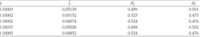
Table 1: Parameter estimates of an Ornstein-Uhlenbeck process with two or three splitting. Five trajectories
are simulated with parametersφ0.1,λ0.05 andπ2π31/2.
ϕ λ π2# π3#
0.10003 0.05139 0.499 0.501
0.10002 0.05152 0.525 0.475
0.10002 0.04974 0.524 0.476
0.10033 0.05028 0.498 0.502
0.10005 0.04852 0.524 0.476
Moreover, we have the following results:
λt−−−→a.s. λ,
#
πnt−→a.s. πn ∀n,
√
mt
λ λt
−1
L
−→N0,1,
√
mt$π#nt−πn
πn1−πn L
−→N0,1, ∀n
5.10
suggesting consistency and asymptotic normality of the estimators in a more general context. We perform a simulation analysis for the model above in the following way.
Equation5.1is discretized as
Xt hXt ϕ
t h
t
Xsds Wt h−Wt. 5.11
For smallhwe take:
Xt h≈Xt ϕhXt ξh, 5.12
whereξh∼N0, h. As initial parameters we take
ϕ0.1,
λ0.05,
π2π3
1 2.
5.13
Acknowledgments
This research has been partially supported by the Natural Sciences and Engineering Research Council of Canada. Also, the authors would like to thank the support received from the Asociaci ´on Mexicana de Cultura
References
1 S. R. Adke and S. R. Dharmadhikari, “The maximum likelihood estimation of coefficient of diffusion
in a birth and diffusion process,” Biometrika, vol. 67, no. 3, pp. 571–576, 1980.
2 L. G. Gorostiza, “A measure valued process arising from a branching particle system with changes
of mass,” in Measure-Valued Processes, Stochastic Partial Differential Equations, and Interacting Systems,
D. A. Dawson, Ed., vol. 5 of CRM Proceedings and Lecture Notes, pp. 111–118, American Mathematical Society, Providence, RI, USA, 1994.
3 T. Huillet, “A branching di usion model of selection: from the neutral wright-fisher case to the one
including mutations,” International Mathematical Forum, vol. 7, no. 1, pp. 1–36, 2012.
4 A. Grigor’yan and M. Kelbert, “Recurrence and transience of branching diffusion processes on
Riemannian manifolds,” The Annals of Probability, vol. 31, no. 1, pp. 244–284, 2003.
5 S. Roelly and A. Rouault, “Construction et propri´et´es de martingales des branchements spatiaux
interactifs,” International Statistical Review, vol. 58, no. 2, pp. 173–189, 1990.
6 S. N. Ethier and T. G. Kurtz, Markov Processes, Wiley Series in Probability and Mathematical Statistics:
Probability and Mathematical Statistics, John Wiley & Sons, New York, NY, USA, 1986.
7 R. Kulperger, “Parametric estimation for simple branching diffusion processes. II,” Journal of
Multivariate Analysis, vol. 18, no. 2, pp. 225–241, 1986.
8 M. J. Phelan, “A Girsanov transformation for birth and death on a Brownian flow,” Journal of Applied
Probability, vol. 33, no. 1, pp. 88–100, 1996.
9 R. H ¨opfner and E. L ¨ocherbach, “On local asymptotic normality for birth and death on a flow,”
Stochastic Processes and their Applications, vol. 83, no. 1, pp. 61–77, 1999.
10 J. Jacod and A. N. Shiryaev, Limit Theorems for Stochastic Processes, vol. 288 of Grundlehren der
Mathematischen Wissenschaften, Springer, Berlin, Germany, 1987.
11 J. Hernandez, P. Olivares, and M. Escobar, “Asymptotic behavior of maximum likelihood estimators
in a branching diffusion model,” Statistical Inference for Stochastic Processes, vol. 12, no. 2, pp. 115–137,
2009.
12 P. Jagers, Branching Processes with Biological Applications, Wiley-Interscience, London, UK, 1975.
13 S. Asmussen and H. Hering, Branching Processes, vol. 3 of Progress in Probability and Statistics,
Birkh¨auser, Boston, Mass, USA, 1983.
14 M. M´etivier, Semimartingales, vol. 2 of de Gruyter Studies in Mathematics, Walter de Gruyter, Berlin,
Germany, 1982.
15 B. L. S. Prakasa Rao, Semimartingales and Their Statistical Inference, vol. 83 of Monographs on Statistics
Submit your manuscripts at
http://www.hindawi.com
Hindawi Publishing Corporation
http://www.hindawi.com Volume 2014
Mathematics
Journal ofHindawi Publishing Corporation
http://www.hindawi.com Volume 2014
Hindawi Publishing Corporation http://www.hindawi.com
Differential Equations
International Journal of
Volume 2014
Applied MathematicsJournal of
Hindawi Publishing Corporation
http://www.hindawi.com Volume 2014
Hindawi Publishing Corporation
http://www.hindawi.com Volume 2014
Hindawi Publishing Corporation
http://www.hindawi.com Volume 2014
Mathematical PhysicsAdvances in
Complex Analysis
Journal ofHindawi Publishing Corporation
http://www.hindawi.com Volume 2014
Optimization
Journal of Hindawi Publishing Corporationhttp://www.hindawi.com Volume 2014
Combinatorics
Hindawi Publishing Corporation
http://www.hindawi.com Volume 2014
International Journal of
Hindawi Publishing Corporation
http://www.hindawi.com Volume 2014
Journal of
Hindawi Publishing Corporation
http://www.hindawi.com Volume 2014
Function Spaces
Abstract and Applied Analysis Hindawi Publishing Corporation
http://www.hindawi.com Volume 2014
International Journal of Mathematics and Mathematical Sciences
Hindawi Publishing Corporation http://www.hindawi.com Volume 2014
The Scientific
World Journal
Hindawi Publishing Corporation
http://www.hindawi.com Volume 2014
Hindawi Publishing Corporation
http://www.hindawi.com Volume 2014
Discrete Dynamics in Nature and Society
Hindawi Publishing Corporation
http://www.hindawi.com Volume 2014 Hindawi Publishing Corporation
http://www.hindawi.com Volume 2014
Discrete Mathematics
Journal ofHindawi Publishing Corporation
http://www.hindawi.com Volume 2014
Hindawi Publishing Corporation
http://www.hindawi.com Volume 2014