Stable finite element methods for the Stokes problem

© Hindawi Publishing Corp.

STABLE FINITE ELEMENT METHODS FOR THE STOKES PROBLEM

YONGDEOK KIM and SUNGYUN LEE

(Received 11 March 1999)

Abstract.The mixed finite element scheme of the Stokes problem with pressure stabi-lization is analyzed for the cross-gridPk−Pk−1elements,k≥1, using discontinuous pres-sures. TheP+

k−Pk−1elements are also analyzed. We prove the stability of the scheme using the macroelement technique. The order of convergence follows from the standard theory of mixed methods. The macroelement technique can also be applicable to the stability analysis for some higher order methods using continuous pressures such as Taylor-Hood methods, cross-grid methods, or iso-grid methods.

Keywords and phrases. Mixed finite element method, stabilization, Stokes problem. 2000 Mathematics Subject Classification. Primary 65N12, 65N15, 65N30.

1. Introduction. For the finite element approximation of the stationary Stokes equations several approaches appear in the literature [6, 9, 13]. The purpose of this paper is to analyze the mixed finite element scheme with pressure stabilization for some higher order triangular elements.

LetΩbe a bounded polygonal domain inR2_{. We consider the approximation of the} stationary Stokes problem: findu=(u1,u2)andpsatisfying

−ν∆u+∇p=f inΩ,

divu=0 inΩ,

u=0 on∂Ω,

(1.1)

whereuis the fluid velocity,pis the pressure,fis the given body force per unit mass, andν >0 is the viscosity. For the sake of simplicity, we take the viscosity equal to one. With the usual notation (see Section 2 for details) the standard variational formulation of this problem is: findu∈H1

0(Ω)2andp∈L20(Ω)such that

(∇u,∇v)−(divv,p)=(f,v), v∈H1 0(Ω)2,

(divu,q)=0, q∈L2 0(Ω),

(1.2)

where(·,·)denote the usualL2_{inner products. Forf∈H}−1_(Ω)2_{this problem has a} unique solution (cf. [9]). The standard mixed method based on (1.2) reads as follows: finduh∈Vh⊂H01(Ω)2andp∈Ph⊂L20(Ω)such that

∇uh,∇v−divv,ph=(f,v), v∈Vh,

Suppose that the finite element spacesVhandPhindexed by the parameterh, 0<h<1, satisfy the inf-sup condition or the Babuška-Brezzi stability condition

inf 0≠p∈Ph

sup

0≠v∈Vh

(divv,p)

v 1 p 0≥C, (1.4)

whereCis a positive constant independent ofh. Then the theory of mixed methods states that the system (1.3) has a unique solution(uh,ph)satisfying

u−uh 1+ p−ph 0≤C

inf

v∈Vh u−v 1+qinf∈Ph p−q 0

, (1.5)

where(u,p)is the solution to (1.2). Introducing the associated bounded bilinear form

B(u,p;v,q)=(∇u,∇v)−(divv,p)+(divu,q), = ±1, (1.6)

and the linear functional

L(v,q)=(f,v), (1.7)

we can recast the formulation (1.3) as follows: find(uh,ph)∈Vh×Phsuch that

Buh,ph;v,q=L(v,q), (v,q)∈Vh×Ph. (1.8)

Then the main result of [1, 2] says that (1.5) holds provided

sup

0≠(v,q)∈Vh×Ph

B(u,p;v,q)

v 1+ q 0≥C

u 1+ p 0, (u,p)∈Vh×Ph, (1.9)

whereCis a positive constant independent ofh. Equation (1.9) will be referred to the stability condition for a bilinear formBin general.

Since it could be a difficult task to verify (1.4) for a particular choice of velocity and pressure approximations, several methods have been developed aiming at sta-bilizing the discrete solution. We introduce an approximation scheme with pressure stabilization as follows: find(uh,ph)∈Vh×Phsuch that

B(uh,ph;v,q)=L(v,q), (v,q)∈Vh×Ph (1.10)

with

B(u,p;v,q)=(∇u,∇v)−(divv,p)+(divu,q)

+β

T∈Γh

hT[[p]],[[q]]T, = ±1,

L(v,q)=(f,v).

(1.11)

Note that this method was considered as a special case of the stabilization procedures in [7, 10].

Pk−Pk−1elements,k≥1 and thePk+−Pk−1elements,k≥2 (see Section 3). To verify the stability condition (1.9), we will combine the ideas of macroelement technique in [15, 16, 17] and the arguments in [8] for Galerkin least squares methods. Then the er-ror estimate (1.5) follows in the usual manner. The macroelement technique can also be applicable to the stability analysis for some higher order methods using continuous pressures, such as Taylor-Hood methods, cross-grid methods, or iso-grid methods.

An outline of the paper is as follows. In Section 2, we develop the stability analysis and the macroelement technique together with the necessary preliminaries. The sta-bility and convergence of various elements mentioned above are shown in Section 3 by an application of the results in Section 2.

2. Macroelement technique and weak stability. LetᏯhbe a partitioning of ¯Ωinto triangles for a bounded polygonal domainΩ⊂R2_{. The triangulation is assumed to be} regular in the usual sense, that is, for someσ >1,

hK≤σ ρK, K∈Ꮿh, (2.1)

wherehK is the diameter of elementKand ρK is the diameter of the largest circle contained in K. The mesh parameterh is given by h=max(hK)and the set of all interelement boundaries will be denoted byΓh. We will not assumeᏯhto be quasi-uniform.

The finite element subspaces ofPk−Plelement are

Vh=v=v1,v2∈H01(Ω)2:vi|K∈Pk(K), i=1,2, K∈Ꮿh,

Ph=p∈L20(Ω):p|K∈Pl(K), K∈Ꮿh, (2.2) wherePs denotes the collection of all polynomials of degree not greater thans and L2

0(Ω)denotes the subspace ofL2(Ω)of functions with zero mean value. Our notation is standard. The norms and seminorms in the Sobolev spacesH1_(Ω)2_{are denoted by} · 1and|·|1, respectively.

Given any regular triangulationᏯh, by amacroelementwe now mean a connected setM of adjoining elementsKfromᏯh. Two macroelementsMand ¯Mare said to be equivalentif there is a continuous one-to-one and onto mappingF:M→M¯such that

F|Kis affine for eachK⊂M. For a macroelementMwedefinethe spacesV0,M andPM consistent withVhandPh:

V0,M=v∈H01(M)2:v|K∈Pk(K)2, K⊂M, (2.3) PM=p∈L20(M):p|K∈Pl(K), K⊂M. (2.4) Further wedefine

NM=p∈PM:(v,∇hp)M=0,v∈V0,M, (2.5)

where∇hp is given by∇p|K on eachK⊂M. The collection of edges of elements in the interior ofMis denoted byΓM. The following seminorms defined inPhturns out to be very useful for the analysis below:

|p|2

h=

K∈Ꮿh h2

K ∇p 20,K, |[[p]]|2h=

T∈Γh

InPM we similarly define

|p|2

M=

K⊂M h2

K ∇p 20,K, |[[p]]|2M=

T∈ΓM

hT[[p]],[[p]]T. (2.7)

Here, the collection of edges of elements in the interior ofMis denoted byΓM, · 0,K is theL2_{norm onK,(·,·)}

Tis the inner product inL2(T ),hTis the diameter ofT, and [[p]]T is the jump inpalongT.

The macroelement technique is based on the macroelement partitioningᏹh satis-fying the following conditions:

(M1) there is a fixed set of equivalence classesᏰi,i=1,...,q, of macroelements such that eachM∈ᏹhbelongs to one ofᏰi;

(M2) there is a positive integerLsuch that eachK∈Ꮿhis contained in at least one and not more thanLmacroelements ofᏹh;

(M3) eachM∈Ᏸi, i=1,...,q,satisfies (M3a) p∈NM implies that|p|M=0.

The usefulness of the macroelement concept and the above mesh-dependent norms is that it enables us to establish some weak stability estimates for the proof of (1.9).

Remark2.1. We have modified the presentation of Sternberg [16, 17] to deal with the pressure stabilization and discontinuous pressure approximations.

Lemma2.2. Let Ᏸ be a class of equivalent macroelements. Suppose that (M3a) is valid for everyM∈Ᏸ. Then there is a constantC >0such that

sup

0≠v∈V0,M

(v,∇hp)M

|v|1,M ≥C|p|M, p∈PM (2.8) holds for allM∈Ᏸ.

Proof. ForM∈Ᏸ, define a scaling invariant

βM= inf

0≠p∈PM

sup

0≠v∈V0,M

(v,∇hp)M

|v|1,M|p|M (2.9) which is positive from the hypothesis. By virtue of the argument of Sternberg (cf. [15, 17]), the regularity condition (2.1) ensures that there is a constantC such that

βM≥C >0 for allM∈Ᏸ,which implies (2.8).

Lemma2.3. Suppose that there is a macroelement partitioningᏹhsatisfying (M1), (M2),and (M3). Then the weak stability inequality

sup

0≠v∈Vh

(divv,p)

v 1 ≥C1|p|h−C2|[[p]]|h, p∈Ph (2.10) is valid.

Proof. The local weak stability estimates (2.8) implies that for a givenp∈Phand M∈ᏹh, there isvM∈VhwithvM=0inΩ\Msuch that

Then we have

divvM,pM= −

vM,∇hpM+

T∈ΓM

vM·n,[[p]]T, (2.13)

divvM,pM≥C|p|2M−

T∈ΓM h−1

T vM 20,T

1/2

|[[p]]|M. (2.14)

Herendenotes a unit normal toT. From Lemma 2.4 we have the estimates

T∈ΓM h−1

T vM 20,T≤C

K⊂M h−2

K vM 20,K≤C|v|21,M. (2.15)

Combining (2.12), (2.14), and (2.15), we obtain

divvM,pM≥C1|p|M2−C2|p|M|[[p]]|M, (2.16) where C1>0 and C2> 0 can be taken independent of M. Next let us define v∈ Vhthroughv=M∈ᏹhvM.Then the macroelement conditions (M1), (M2), (M3), and

(2.16) give

(divv,p)= M∈ᏹh

divvM,pM

≥C1

M∈ᏹh

|p|2

M−C2

M∈ᏹh

|p|M|[[p]]|M

≥C1|p|2h−C2

M∈ᏹh

|p|2

M

1/2

M∈ᏹh

|[[p]]|2

M

1/2

≥C1|p|2h−C2 √

L|p|h √

L|[[p]]|h

=C1|p|2h−C2L|p|h|[[p]]|h.

(2.17)

Since

v 1≤C|v|1≤C

M∈ᏹh

|vM|1,M≤C

M∈ᏹh

|p|M

≤CL K∈Ꮿh

hK ∇p 0,K≤CL|Ω|1/2|p|h,

(2.18)

it follows from (2.17) that there are constantsC1>0 andC2>0 satisfying (2.10). Here |Ω|denotes the measure ofΩ.

Lemma2.4. LetMbe a macroelement. Then we have foru∈Vh,

T∈ΓM h−1

T u 20,T ≤C

K⊂M h−2

K u 20,K, (2.19)

and foru∈V0,M,

K⊂M h−2

Proof. According to the argument of [3, page 1045] it is not difficult to see that foru∈Vh0,

T∈∂K h−1

T u 20,T≤Ch−2K u 20,K. (2.21)

Then (2.19) follows immediately. Next, applying the argument of a proof of the inverse inequality for piecewise polynomials (cf. [13, page 195]), we can show that (2.20) holds foru∈V0,M.

Lemma2.5. Suppose that either k≥2in the definition (2.2) of Vh orPh⊂C(Ω). Then there are two positive constantsC1andC2such that

sup

0≠v∈Vh

(divv,p)

v 1 ≥C1 p 0−C2|p|h, p∈Ph. (2.22)

Proof. These are the cases (i) and (ii) of [8, Lemma 3.3]. See [8, pages 1685–1687] for the proof.

Lemma2.6. Under the assumption of Lemma 2.3 there are two positive constants

C1andC2such that the weak stability inequality

sup

0≠v∈Vh

(divv,p)

v 1 ≥C1 p 0−C2|[[p]]|h, p∈Ph (2.23) holds.

Proof. Equation (2.23) follows from (2.10) and (2.22). To be more precise, letC1,C2 andc1,c2be the constants in (2.10) and (2.22), respectively. For 0< t <1 we have

sup

0≠v∈Vh

(divv,p)

v 1 ≥(1−t)

C1|p|h−C2|[[p]]|h+tc1 p 0−c2|p|h ≥tc1 p 0+(1−t)C1−tc2|p|h−(1−t)C2|[[p]]|h.

(2.24)

Then (2.23) follows providedt < C1(C1+c2)−1.

We are ready to verify the stability condition (1.9) for the method (1.10). We do the case=1.The other case= −1 is similar.

Theorem2.7. Suppose that there is a macroelement partitioning ᏹh satisfying (M1),(M2),and (M3) for a regular triangulationᏹh of Ω⊂R2. Then given a stabi-lization parameterβ >0the stability condition (1.9) for the method (1.10) is valid.

Proof. Let(u,p)∈Vh×Ph.First, we note that

B(u,p;u,p)= ∇u 2

0+β|[[p]]|2h≥C1 u 21+β|[[p]]|2h. (2.25) Next, according to (2.23), there isw∈Vhsatisfying

and w 1= p 0.Then fort1>0 andt2>0,

B(u,p;−w,0)= −(∇u,∇w)+(divw,p)

≥ − u 1 p 0+C2 p 02−C3 p 0|[[p]]|h ≥

C2−t₂1−C3₂t2 p 20− u 2 1 2t1 −

C3|[[p]]|2h 2t2 .

(2.27)

Choosingt1andt2small enough, we have

B(u,p;−w,0)≥C4 p 20−C5 u 21−C6|[[p]]|2h (2.28) for some positive constantsC4,C5, andC6.Let us denote(v,q)=(u−δw,p). It follows from (2.25) and (2.28) that

B(u,p;v,q)=B(u,p;u,p)+δB(u,p;−w,0)

≥δC4p20+

C1−δC5u21+

β−δC6[[p]]2h.

(2.29)

Choosing 0< δ <minC1C5−1,βC6−1we obtain

B(u,p;v,q)≥C7 u 1+ p 02 (2.30) for some positive constantC7. On the other hand, we have

v 1+ q 0≤C8 u 1+ p 0 (2.31) for some positive constant C8. Finally combining (2.30) and (2.31) we establish the stability condition (1.9) for the method (1.10).

The error estimates are now obtained in the usual manner from the stability inequal-ity (1.9) and from the following estimates (cf. [8, 9]):

K∈Ꮿh h2

K ∇q 20,K+

T∈Γh

hT([[q]],[[q]])T

1/2

≤C q 0, q∈Ph, (2.32)

inf q∈Ph

K∈Ꮿh h2

K ∇(q−p) 20,K+

T∈Γh

hT([[q−p]],[[q−p]])T

1/2

≤C inf

q∈Ph q−p 0≤Ch l+1_|p|

l+1, p∈Hl+1(Ω),

(2.33)

inf

v∈Vh u−v 1≤Ch k_|u|

k+1, u∈Hk+1(Ω)2. (2.34)

Theorem2.8. Let the assumptions of Theorem 2.7 be valid. Assume further that the solution(u,p)to (1.2) satisfiesu∈Hk+1_(Ω)2 _andp∈Hl+1_{(Ω). Then forβ >0,} (1.10) has a unique solution(uh,ph)satisfying (1.5) and

u−uh 1+ p−ph 0≤Chk|u|k+1+hl+1|p|l+1. (2.35) If in additionΩis a convex polygon,then we have

Proof. We follow the argument of [8, page 1688]. Let ˜u∈Vhand ˜p∈Phbe the interpolants ofu and p, respectively. The stability condition (1.9) ofB implies the existence of(v,q)∈Vh×Phsuch that

v 1+ q 0≤C,

_{u˜−uh1+p˜−ph0≤B}

uh−˜u,ph−p˜;v,q. (2.37)

Since

Buh−˜u,ph−p˜;v,q=Bu−˜u,p−p˜;v,q, (2.38)

Bu−u˜,p−p˜;v,q≤C

u−˜u 2

1+ p−p˜ 20+

T∈Γh

hT[[p−p]],[[p˜ −p]]˜ T 1/2

·

v 2

1+ q 20+

T∈Γh

hT[[q]],[[q]]T 1/2

,

(2.39)

we get, from (2.32), (2.33), and (2.37), _{u˜−uh1+p˜−ph0≤C}

u−u˜ 1+ p−p˜ 0, (2.40) which gives (1.5) with the aid of the triangle inequality. Now (2.35) follows from (1.5), (2.33), and (2.34). Moreover, (2.36) follows from the Aubin-Nitsche argument using the a priori estimate [12],

u 2+ p 1≤C f 0 (2.41)

for a convex polygon.

3. Higher order stable elements. In this section, we apply, essentially, Theorems 2.7 and 2.8 for the analysis of several higher order stable elements. We will verify the macroelement conditions (M1), (M2), and (M3) and the approximation properties (2.33) and (2.34) for each method to establish the error estimates (2.35) and (2.36). Our main concern is the verification of the condition (M3), since a construction of macroelement partitioning satisfying (M1) and (M2) is not difficult and the approximation properties (2.33) and (2.34) follow from the standard interpolation theory. For the P+

k −Pk−1 elements,Vhis enlarged using bubble functions on certain triangles. For thePk−Pk cross-grid elements or thePk−Pkiso-grid elements, the pressure triangulationᏯhor ˜

Ꮿhis coarser than the velocity triangulationᏯh. But the results of Section 2 can be interpreted without difficulty.

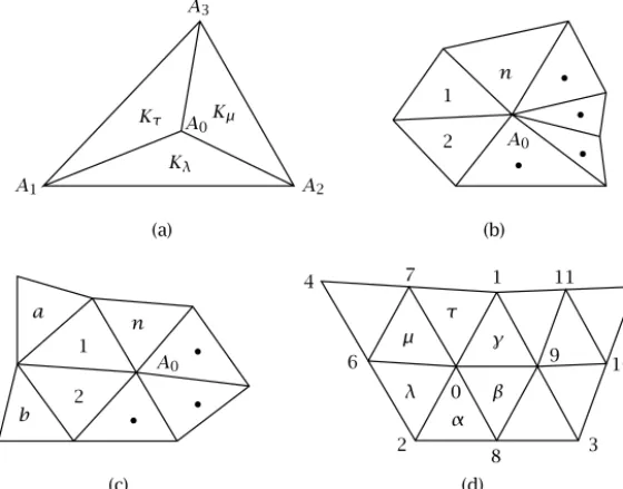
We begin by recalling that the barycentric coordinatesλi=λi(x), 1≤i≤3,ofx= (x,y)∈R2_{with respect to the pointsAi=(xi,yi), 1≤i≤3, which makes a triangle}

K, are the unique solution of the linear system

3

i=1

λiAi=x,

3

i=1

(a) A3

A2 A1

Kλ

A0 Kτ Kµ

(b)

• •

• •

A0 2

1 n

(c) a

b 2

1

•

n

A0 •

•

(d)

4 7 1 11 ₅

10

3 8

2

6 γ 9

τ µ

λ 0 α

β

Figure3.1. Examples of macroelement.

It follows that

λ1

λ2

= 1

|K|

y2−y3 −x2−x3 −y1−y3 x1−x3

x−x3

y−y3

, (3.2)

where|K|denotes the measure ofKand= ±1 depending on the orientation ofA1,A2, andA3. Similar relations hold also for

_λ1 λ3

andλ2λ3

. Note that for any nonnegative integersi,j,k,

Kλ i

1λj2λk3dx=_(i+2_ji₊!j_k!k₊!_2)!|K|. (3.3) A few examples of macroelement are illustrated in Figure 3.1. For the macroelement in Figure 3.1a we interpret byλ0,λ1,λ2the barycentric coordinates onKλwith respect to A0,A1, andA2. The similar interpretation of notation will apply for the other figures. 3.1. The cross-gridPk−Pk−1elements,k≥1, using discontinuous pressures. In the cross-grid methods using discontinuous pressures the triangulationᏯhis obtained from a triangulation Ꮿ

hby dividing each K∈Ꮿh into three triangles inserting an interior vertexA0as in Figure 3.1a, whereA0is not necessarily the center of gravity ofK_{. Fork≥1 we defineVhby (2.2) and}

Ph=p∈L20(Ω):p|K∈Pk−1(K), K∈Ꮿh. (3.4) Lemma3.1. Let M be a macroelement consisting of three triangles aligned as in Figure 3.1a. DefineV0,Mby (2.3) and

Proof. Letp∈NM and write

px|Kλ=

gλ0,λ1,λ2

|Kλ| . (3.6)

Suppose thatpx|Kµ=h(µ0,µ3,µ2)/|Kµ|. Hereλi’s andµj’s are the barycentric

coordi-nates ofKλandKµ, respectively. Chooseu=(u1,0)∈Vh,Msuch that

u1=

        

λ0λ2(g+h)λ0,λ1,λ2 inKλ, µ0µ2(g+h)µ0,µ3,µ2 inKµ,

0 otherwise.

(3.7)

Then(u,∇hp)M=0 gives an equation

λ0λ2(g+h)λ0,λ1,λ2,g

λ0,λ1,λ2 |Kλ| _Kλ+

µ0µ2(g+h)µ0,µ3,µ2,h

µ0,µ3,µ2 |Kµ| _Kµ=0.

(3.8)

On the other hand, it is not difficult to see from (3.3) that 1

Kλ

Kλ

λ0λ2g2+ghλ0,λ1,λ2dx=_K1

µ

Kµµ0µ2

g2_+ghµ

0,µ3,µ2dx. (3.9) Combining (3.8) and (3.9) we get

1

Kµ

Kµµ0µ2(g+h)

2_µ

0,µ3,µ2dx=0 (3.10) which implies

(g+h)µ0,µ3,µ2=0. (3.11) Then we have

px|Kµ= −g

µ0,µ3,µ2

|Kµ| . (3.12)

By the same argument we obtain

px|Kτ=

gτ0,τ3,τ1

|Kτ| , px|Kλ= −

gλ0,λ2,λ1

|Kλ| . (3.13)

Thusgis a polynomial satisfying

gλ0,λ1,λ2= −gλ0,λ2,λ1,

gµ0,µ2,µ3= −gµ0,µ3,µ2,

gτ0,τ3,τ1= −gτ0,τ1,τ3.

(3.14)

Let us consider the casek=4 first before we turn to the general casek≥1. From (3.6), (3.14), and the assumptionk=4, we can write

px|Kλ= a

|Kλ|

λ2 1−λ22

+_|Kb

λ|

with two parametersaandbinR. Similarly,py|Kλ can be written as the right-hand

side of (3.15) with the parametersaandbreplaced bya_{andb, respectively. Note} also thatpxandpy inKµorKτcan be expressed usinga,banda,b, respectively. Then from (3.6), (3.15), and

pxy=

pyx (3.16)

which are valid on eachK∈Ꮿh, we get

aλ1,y−λ2,y=aλ1,x−λ2,x, bλ1,y−λ2,y=bλ1,x−λ2,x. (3.17)

Applying (3.2) and (3.17) inKλ,Kµ, orKτ, we find that(a,a)and(b,b)satisfies the homogeneous system in(s,t),

sx1−x0+ty1−y0=0, sx2−x0+ty2−y0=0, (3.18)

of which the solution is trivial since the determinant of the coefficient matrix is equal to|Kλ|/2>0. This implies that|p|M =0 whenk=4. For the general casek≥2, we can write

px|Kλ=

1 |Kλ|

i+j+l=k−2

i≥j≥0, l≥0

ai,j,lλi1λj2−λi2λj1

λl

0. (3.19)

Similarly,py|Kλ can be written as the right-hand side of (3.19) with the parameters ai,j,lreplaced byai,j,l. Moreoverpxandpy inKµorKτcan be expressed usingai,j,l anda

i,j,lanalogously. Then we find that(ai,j,l,ai,j,l)satisfies (3.18) for eachi,j,l. It follows thatai,j,l=ai,j,k,l=0 for eachi,j,land that∇p|K=0, for allK⊂M. This completes the proof.

Thus we have a nonoverlapping macroelement partitioning, with one class of macroelements equivalent toK_∈Ꮿ

h, which satisfies (M1), (M2), and (M3). A care-ful observation of the analysis of Section 2 also shows that for a nonoverlapping macroelement partitioning the coefficient ofβin the approximation scheme (1.10) can be reduced to

K_∈Ꮿ h

T∈ΓK

hT[[p]],[[q]]T, (3.20)

Theorem3.2. Suppose thatᏯh,which is obtained fromᏯh,is a regular triangula-tion ofΩ. Fork≥1,defineVhandPhby (2.2) and (3.4),respectively. Then Theorem 2.8 is valid withβ >0for the approximation scheme (1.10) or for the locally stabilized approximation scheme.

Remark3.3. The casek=1 can be considered as a special case of the scheme in [11].

3.2. TheP+

k−Pk−1elements,k≥2, using discontinuous pressures. The argument of Lemma 3.1 shows that in general a macroelementMof type (b) in Figure 3.1 con-sisting ofntriangles with a common vertexA0in the interior ofM satisfies (M3a) providednis odd. When the indexnofA0is even, we augment bubble functions on a triangle inMin order to verify (M3a). For a regular triangulationᏯhofΩ, we can construct a macroelement partitioningᏹh, consisting of macroelements of type (b) and (c) in Figure 3.1. LetᏱbe a set of triangles inᏯhsuch that for each macroelement M∈ᏹhwith an interior vertex of even index there is a triangleK∈Ᏹ. Then we have the following result forP+

k−Pk−1element.

Theorem3.4. Suppose thatᏯhis a regular triangulation ofΩ. Define

Vh=v∈H01(Ω)2:v|K∈Pk(K)2, K∈Ꮿh; v|K∈[Pk(K)⊕λ1λ2λ3Pk−2(K)]2, K∈Ᏹ,

Ph=p∈L20(Ω):p|K∈Pk−1(K), K∈Ꮿh.

(3.21)

Hereλ1,λ2,λ3are the barycentric coordinates of the corresponding triangleK. Then Theorem 2.8 is valid fork≥2.

3.3. The cross-gridPk−Pkelements,k≥1. In the cross-gridPk−Pkelements,k≥1, the triangulationᏯhfor velocity is obtained from the triangulation ˜Ꮿhfor pressure by dividing each ˜K∈Ꮿ˜h into three triangles inserting an interior vertex A0 as in Figure 3.1a, whereA0is not necessarily the center of gravity of ˜K.

Fork≥1 we defineVhby (2.2) and

Ph=p∈L20(Ω):p|K˜∈Pk(K),˜ K˜∈Ꮿ˜h. (3.22)

Lemma3.5. Let M be a macroelement consisting of three triangles aligned as in Figure 3.1a. DefineV0,Mby (2.3) and

PM=p∈Pk(M) fork≥1. (3.23)

Then (M3a) is valid.

Proof. Letp∈NM and chooseu∈V0,Msuch that

u=         

λ0∇p inKλ, µ0∇p inKµ, τ0∇p inKτ.

Then(u,∇hp)M=0 gives

λ0∇p,∇pKλ+

µ0∇p,∇pKµ+

τ0∇p,∇pKτ=0 (3.25)

which implies∇p|K=0 for allK⊂Mand thus|p|M=0.

Thus we have a nonoverlapping partitioning, with one class of macroelements equiv-alent to (a) in Figure 3.1, satisfying (M1), (M2), and (M3). Since the approximation prop-erties (2.33) and (2.34) are valid, we obtain the following result for the cross-gridPk−Pk elements,k≥1.

Theorem3.6. Suppose thatᏯh,which is obtained fromᏯ˜h,is a regular triangula-tion ofΩ. Fork≥1,defineVhandPhby (2.2) and (3.22),respectively. Then Theorem 2.8 is valid withβ=0.

3.4. The iso-grid Pk−Pk elements, k≥ 1, using continuous pressures. In the Pk−Pk iso-grid elements,k≥ 1, using continuous pressures, the triangulationᏯh for velocity is obtained from a triangulation ˜Ꮿhfor pressure by dividing each ˜K∈Ꮿ˜h into four triangles inserting three vertices, one at each edge of ˜K. Each of the inserted vertices is not necessarily a mid-point of the corresponding edge. Fork≥1 we define Vhby (2.2) and

Ph=p∈L20(Ω)∩C(Ω):p|K˜∈Pk(K),˜ K˜∈Ꮿ˜h. (3.26) Lemma3.7. LetM be a macroelement consisting of twelve triangles aligned as in Figure 3.1d. Define

V0,M=v∈H01(M)2:v|K∈Pk(K)2, K∈Ꮿh∩M,

PM=p∈C(M):p|K˜∈Pk(K),˜ K˜∈Ꮿ˜h∩M fork≥1. (3.27) Then (M3a) is valid.

Proof. Letp∈NM and define

g=                                   

τ0 inK017,

µ0 inK076,

λ0 inK062,

α0 inK028,

β0 inK089,

γ0 inK091, 0 otherwise,

(3.28)

whereKijkdenotes the triangle with verticesAi,Aj, andAk. Lete=(e1,e2)be the unit vector in the direction ofA1A→2, and chooseu=(e1gpe,e2gpe)∈V0,M. Note that pe= ∇p·eis continuous onK123∪K142. Then(u,∇hp)M=0 gives

τ0pe,peK017+

µ0pe,peK076+···+

which impliespe|K017=0,...,pe|K091=0. The similar argument gives alsopd|K091=0, wheredis the unit vector in the direction ofA2A→4. Sinceeanddare linearly indepen-dent, we get∇p|K091 =0 and so∇p|K123=0. Next consideru=(e2gpe⊥,−e1gpe⊥)∈

V0,M, wherep⊥e ∈Pk−1(R2)is the extension of(e2px−e1py)|K142. Then(u,∇hp)M=0 gives

τ0pe⊥,pe⊥K017+

µ0p⊥e,p⊥eK076+

λ0pe⊥,p⊥eK062=0 (3.30) which impliesp⊥

e|K062=0. Since(e1,e2)and(e2,−e1)are orthogonal,pe|K062=p⊥e|K062 =0 implies ∇p|K062 = 0 and so ∇p|K142 =0. The analogous argument also gives ∇p|K135=0. It follows that|p|M=0.

Now it is easy to construct a macroelement partitioning, with only one class of macroelements equivalent to (d) in Figure 3.1, satisfying (M1), (M2), and (M3). Since the approximation properties (2.33) and (2.34) are valid, we have the following result for the iso-gridPk−Pkelements,k≥1, using continuous pressures.

Theorem3.8. Suppose thatᏯh,which is obtained fromᏯ˜h,is a regular triangula-tion ofΩ. Fork≥1,defineVhandPhby (2.2) and (3.26),respectively. Then Theorem 2.8 is valid withβ=0.

3.5. ThePk−Pk−1Taylor-Hood elements,k≥2

Lemma3.9. Let M be a macroelement consisting of three triangles aligned as in Figure 3.1a. DefineV0,Mby (2.3) and

PM=p∈C(M):p|K∈Pk−1(K), K⊂M fork≥2. (3.31)

Then (M3a) is valid.

Proof. Lete=(e1,e2)be the unit vector in the direction of A0A→2. Chooseu=

(u1,u2)∈V0,M such that

u1=

        

e1λ0λ2pe inKλ, e1µ0µ2pe inKµ,

0 inKτ,

u2=

        

e2λ0λ2pe inKλ, e2µ0µ2pe inKµ,

0 inKτ,

(3.32)

wherepe= ∇p·e. Letp∈NM. Then(u,∇hp)M=0 gives

λ0λ2pe,peKλ+

µ0µ2pe,peKµ=0 (3.33)

which impliespe|Kλ=0 andpe|Kµ =0. Similarly, we havepd|Kλ=0 andpd|K3=0,

wheredis the unit vector in the direction ofA0A→3. Sinceeanddare linearly indepen-dent, we have∇p=0 inKµ. By the same reasoning we also have∇p=0 inKλorKτ. It follows that|p|M=0.

Theorem3.10. Suppose thatᏯhis a regular triangulation ofΩ. Fork≥2,define

Vhby (2.2) and

Ph=p∈L20(Ω)∩C(Ω):p|K∈Pk−1(K), K∈Ꮿh. (3.34) Then Theorem 2.8 is valid withβ=0.

Remark3.11. It should be pointed out that some restrictions (cf. [5]) inherited from the result of Scott and Vogelius [14] are removed here. See [4] for a differ-ent proof.

Acknowledgement. This work was supported in part by KAIST.

References

[1] I. Babuška,Error-bounds for finite element method, Numer. Math.16(1970/1971), 322– 333. MR 44#6166. Zbl 214.42001.

[2] I. Babuška and A. K. Aziz,Survey lectures on the mathematical foundations of the finite element method, The Mathematical Foundations of the Finite Element Method with Applications to Partial Differential Equations (Proc. Sympos., Univ. Maryland, Bal-timore, Md., 1972) (New York), Academic Press, 1972, With the collaboration of G. Fix and R. B. Kellogg, pp. 1–359. MR 54#9111. Zbl 268.65052.

[3] I. Babuška, J. Osborn, and J. Pitkäranta, Analysis of mixed methods using mesh de-pendent norms, Math. Comp. 35 (1980), no. 152, 1039–1062. MR 81m:65166. Zbl 472.65083.

[4] D. Boffi,Stability of higher order triangular Hood-Taylor methods for the stationary Stokes equations, Math. Models Methods Appl. Sci. 4 (1994), no. 2, 223–235. MR 95h:65079. Zbl 804.76051.

[5] F. Brezzi and R. S. Falk,Stability of higher-order Hood-Taylor methods, SIAM J. Numer. Anal.28(1991), no. 3, 581–590. MR 91m:65272. Zbl 731.76042.

[6] F. Brezzi and M. Fortin,Mixed and Hybrid Finite Element Methods, Springer Series in Com-putational Mathematics, vol. 15, Springer-Verlag, New York, 1991. MR 92d:65187. Zbl 788.73002.

[7] J. Douglas, Jr. and J. P. Wang,An absolutely stabilized finite element method for the Stokes problem, Math. Comp.52(1989), no. 186, 495–508. MR 89j:65069. Zbl 669.76051. [8] L. P. Franca and R. Stenberg,Error analysis of Galerkin least squares methods for the elas-ticity equations, SIAM J. Numer. Anal.28(1991), no. 6, 1680–1697. MR 92k:73066. Zbl 759.73055.

[9] V. Girault and P.-A. Raviart,Finite Element Methods for Navier-Stokes Equations, Theory and Algorithms, Springer Series in Computational Mathematics, vol. 5, Springer-Verlag, Berlin, New York, 1986. MR 88b:65129. Zbl 585.65077.

[10] T. J. R. Hughes and L. P. Franca,A new finite element formulation for computational fluid dynamics. VII. The Stokes problem with various well-posed boundary con-ditions: symmetric formulations that converge for all velocity/pressure spaces, Comput. Methods Appl. Mech. Engrg.65 (1987), no. 1, 85–96. MR 89j:76015g. Zbl 635.76067.

[11] N. Kechkar and D. Silvester, Analysis of locally stabilized mixed finite element meth-ods for the Stokes problem, Math. Comp.58(1992), no. 197, 1–10. MR 92e:65138. Zbl 738.76040.

[14] L. R. Scott and M. Vogelius,Norm estimates for a maximal right inverse of the divergence operator in spaces of piecewise polynomials, RAIRO Modél. Math. Anal. Numér.19 (1985), no. 1, 111–143. MR 87i:65190. Zbl 608.65013.

[15] R. Stenberg,Analysis of mixed finite elements methods for the Stokes problem: a unified approach, Math. Comp.42(1984), no. 165, 9–23. MR 84k:76014. Zbl 535.76037. [16] ,Error analysis of some finite element methods for the Stokes problem, Math. Comp.

54(1990), no. 190, 495–508. MR 90h:65189. Zbl 702.65095.

[17] ,A technique for analysing finite element methods for viscous incompressible flow, Internat. J. Numer. Methods Fluids11(1990), no. 6, 935–948, The Seventh Inter-national Conference on Finite Elements in Flow Problems (Huntsville, AL, 1989). MR 91k:76112. Zbl 704.76017.

Yongdeok Kim: Department of Mathematics, KAIST, Taejon,305-701, Korea E-mail address:[email protected], [email protected]