Standard Cosmological Models with
Λ
>
0
Paulo Aguiar
Faculdade de Ciˆencias da Economia e da Empresa, Universidade Lus´ıada - Norte, Rua Dr. Lopo de Carvalho, 4369-006 Porto, Portugal
Copyright c2017 by authors, all rights reserved. Authors agree that this article remains permanently open access under the terms of the Creative Commons Attribution License 4.0 International License
Abstract
In this paper we show that the cosmological standard models can describe our universe very realistic way if we add a positive value of the cosmological constant, without the need for the introduction of cold dark matter. Also we clarify that it is physically allowed objects to move in the Universe at speeds greater than light speed without violation of Einstein’s postulates.Keywords
Standard Cosmological Models, Cosmo-logical Constant, Cold Dark Matter, Einstein’s Postulates, Isotropization, Hubble Constant1
Introduction
Standard cosmological models (Friedmann-Lemaˆıtre-Robertson-Walker - FLRW) are often considered by many authors for the particular value of the cosmological constant Λ = 0.
Despite the problem of Einstein’s introduction of this con-stant, because he initially formulates a static model contain-ing matter and then leaves it after the confirmation of the ex-pansion of the Universe, we know that the more general form of relativistic theory of gravitation has aΛterm. Thus, it is arbitrary to fix the value of the cosmological constant before-hand.
From the observational point of view, the classical tests of Einstein’s theory impose an upper limit forΛ. The most stringent test results from observation of the Mercury peri-helion advance is about10−45cm−2(Rindler) [1].
Unfortu-nately this upper limit is too high when we consider the con-straints of the cosmological data, which impose limits many orders of magnitude lower than the previous one, typically Λ≈3H02/c2 ≈10−56 cm−2, whereH
0is the current value
of the Hubble constant andcis the light speed in the empty space. However, even a very small value ofΛ, can play a decisive role in Cosmology.
As has also been discussed previously, the problem that puts the need for the introduction of a (positive) cosmological
constant is related to the age of the oldest structures in the Universe. We know that models withΛ = 0haveH0t0 ≤1,
being 1 only for the limit case ofΩ0= 0. IfH0is sufficiently
large, the age of the globular swarms is incompatible with the age of the universe for any model withΛ = 0.
Here we intend to revert the study of the cosmological con-stant and not the Hubble concon-stant, in a scenario of an expand-ing universe. Recent observational papers that best highlight the need for Λ >0 are: (Perlmuter) [2] and (Riess) [3, 4], which point to values of Hubble constantH0 = 60−75Km
s−1Mpc−1.
There are other arguments in favor of models withΛ6= 0. In the last decade the theory of inflation has appeared to solve some problems of the standard model not yet solved (Starobinsky), [5], (Guth) [6], (Albrecht) [7], [8]. The Eu-clidean casek = 0is strongly favored in this scenario. The modelΛ = 0(Ω0 = 1) givesH0t0 = 2/3. If we consider
the lowest estimates for the lowest globular swarms,t0= 15
Gyears (Sandage) [9], t0 = 15−16Gyears (Primack) [10]
and references thereof,h=H/100should be less than 0.43. This value is currently below the minimum limits of the Hub-ble constant estimate. However, the H0 values within the
range obtained by the observational data (H0 = 60−75Km
s−1Mpc−1) may imply a non-zero cosmological constant.
Of course, the introduction of a third parameter in cos-mological models can produce models with arbitrarily large ages. We’ll check what kind of models can be produced and set the allowed range of values toΛfreeing them from time-scale problems. Thus, it will be necessary to compare the forecasts obtained with the observational data.
Robertson, however, considered cosmological models with evolution and a non-zero cosmological constant, later Stabell and Refsdal [12] presented an identical classification scheme, usingΩ0andq0as free parameters. Almost simultaneously,
but a little later, Glanfield [13] seemingly unaware of Robert-son’s work, published a discussion for models with Λ 6= 0 usingΩ0as ranking parameters. Later, Robertson and
Noo-nan [14] presented a different analysis for cosmological mod-els with cosmological constants using two different combi-nations ofΩΛ0 andΩ0 as parameters. This representation is
the midst of evolutionary models.
Glanfield’s results seem more complete than those of Robertson’s first work. However, in Robertson’s classifi-cation there is only one particular value of the cosmologi-cal constant, currently identified with the value of Einstein’s static model,ΛE, which separates different types of models.
However, Glanfield found that there are in fact two critical values forΛand obtained some particular results for differ-ent values ofΩ0. Their conclusions were most recently
high-lighted by Felten and Isaacman in their review article, where they also discussed the presence of some incorrect aspects in the usual presentation of models withΛ 6= 0. In particular, they have shown that neither of the two critical values ofΛ coincides withΛE.
We also intend to review the models withΛ6= 0and their classification. Let us also calculate the critical values ofΛ which can be expressed analytically. Thus, we have consid-ered some time scale arguments to show that the range of values of the cosmological constant is relatively restricted, so only a reduced region of the plane (Ω0,Λ) should be
ex-plored to compare the theoretical predictions with observa-tional data.
2
FLRW models with
Λ
6
= 0
Let us only consider Friedmann’s cosmological models (with zero pressure) with a cosmological constant. The met-ric for these homogeneous and isotropic models is
ds2=−dt2+a2(t)
dr2 1−kr2 +r
2
dθ2+ sin2θdφ2
. (1) Einstein’s equations
Rab−
1
2Rgab+ Λgab= 8πGTab, (2) allow to obtain the equation
˙ a2 a2 =
8πG 3 ρ−
kc2 a2 +
Λ
3, (3)
involving only the first derivative of the scale factor in cosmic time that will be used in conjunction with conservation con-ditionρa3=const.(which is valid for the matter dominated time) and with the red-shift equation1 +z=a0/a(t).
Divid-ing both members of the previous equation bya˙2/a2 ≡H2, whereHrepresents the Hubble parameter, we obtain
Ω + Ωk+ ΩΛ= 1, (4)
where
Ω≡8πGρ3H2 (5)
represents the matter density, Ωk≡ −
kc2
a2H2 (6)
represents the density due to spatial curvature and ΩΛ≡
Λ
3H2 (7)
represents the density relative to the cosmological constant. Again using the variable y = a(t)/a0 and the three density
parameters evaluated for the current timet0, the equation (3)
takes the form
˙ y=±H0
s
Ω0
1
y−1
+ ΩΛ0(y2−1) + 1. (8)
The equation (8) has an initial ambiguity (±), but now the ob-servational evidence points to the expansion of the Universe (y >˙ 0) and so this ambiguity disappears. We thus only have two parameters: the matter density (Ω0) and that due to the
cosmological constant (ΩΛ0).
Before starting to classify the models with Λ 6= 0, let’s briefly mention the properties of the models for the caseΛ = 0. In this particular situation the equation (8) takes the form
˙ y=H0
s
Ω0−(Ω0−1)y
y (9)
and there is only one classification parameter, Ω0. When
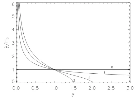
Ω0<1,y˙is defined for all values ofyand tends to√1−Ω0
for large values of y. Herey˙ decreases and tends asymp-totically to the aforementioned value (open universes). For Ω0 > 1we havey˙ = 0forym = Ω0/(Ω0−1). From this
point, the model begins the contraction phase returning to y= 0(closed universes). Note that forΩ0>1,ymis always
greater than 1 and the end of an expansion phase of a cycle happens fora(t) > a0, that is, in the future (see Figure 1).
The half-expansion cycle has a finite duration, except for the limiting case ofΩ0 = 1, for whichy˙will vanish in infinite
[image:2.595.330.545.492.660.2]time (flat universes).
Figure 1. Evolution of the expansion rate as a function of the scale factor, for models withΛ = 0. The numbers in the figure correspond to values of
Ω0.
WhenΛ6= 0the situation is more complicated to analyze. In the Robertson method the behavior of the curvea˙ = 0in the plane (a,Λ) was considered. For this he placeda˙ = 0in the equation (3) as the starting point, obtaining
Λa2 3 +
C
whereC= 8πGρa3/(3). For no pressure models, which we are considering here, the conservation equation is fixed and Cis a constant for a given model. But this constant changes with the model. In fact, since there are only three free pa-rameters, fixingCandk we are forcing a relation between the cosmological parameters that impose constraints in the equation (3) and change its meaning. This is the reason, al-ready discussed by Glanfield [13], which leads us to make this classification using the equation (8) that assumes a differ-ent form from Robertson’s and is reproduced in some articles and books. This is also the technical reason for the problem discussed by Felten and Isaacman [15], where it is stated that, contrary to Robertson’s scheme, the critical value they found does not correspond toΛE(see below).
In this work, we start directly from the equation (8). Since the model will be defined only wherey˙is set, the problem is reduced by finding two zeros off(y) = ΩΛ0y
3
−(Ω0+ ΩΛ0−
1)y+Ω0(withy6= 0). This is a third degree function, its roots
can be expressed analytically using the formula obtained first by Vi`ete in 1615 (referenced in Press [16]).
DefiningQ= (Ω0+ ΩΛ0−1)/(3ΩΛ0)andP= Ω0/(2ΩΛ0),
f(y)will have one or three real roots forQ3−P2 < 0or Q3−P2≥0, respectively. Thus, for a given value of the mat-ter density paramemat-ter, there will be critical values for the cos-mological constant separating regions with a different num-ber of real roots off(y). These particular values ofΛare solutions of the boundary conditionQ3−P2= 0, which cor-responds to
(Ω0+ ΩΛ0−1)
3
27Ω3 Λ0
= Ω
2 0
4Ω2 Λ0
. (11)
Note that the equation above is equivalent to the well-known Glanfield equation [13]
(Ω0+ ΩΛ0−1)
3= (27/4)Ω2
0ΩΛ0, (12)
except forΩΛ0 = 0.
Equation (11) is again a cubic equation and its roots can be determined using the Vi`ete formula. There is a real root if Ω0<1/2and three roots ifΩ0≥1/2. The real root will be
given by
ΩΛc =
3Ω0
2
"s
(Ω0−1)2
Ω2 0
−1 +1−Ω0 Ω0
#1/3
+ 1
q
(Ω0−1)2/Ω20−1 + (1−Ω0)/Ω0
1/3
− (Ω0−1), (13)
forΩ0<1/2, whereas forΩ0≥1/2the roots are given by
ΩΛI = −3Ω0cos
θ 3
−(Ω0−1), (14)
ΩΛc = −3Ω0cos
θ+ 2π 3
−(Ω0−1), (15)
ΩΛM = −3Ω0cos
θ+ 4π 3
−(Ω0−1), (16)
with
θ= cos−1Ω0−1
Ω0
.
We can easily see that forΩ0 = 1/2both equations (13)
and (15) have the same valueΩΛc = 2. This is why we use
the same symbol for these expressions.
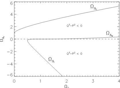
The solutions (13) to (16) are boundaries between regions with sign other thanQ3−P2, that is, with one or three real roots off(y). Figure 2 shows these solutions where we also denote the zones with Q3−P2 < 0. As seen in the this figure,ΩΛc ≥1andΩΛM <ΩΛc. Only forΩ0 ≥1we have
[image:3.595.317.526.255.408.2]ΩΛM ≥0. Finally,ΩΛIis always negative.
Figure 2. Critical values ofΩΛ0. The regions marked withQ
3
−P2 <0
correspond to models for whichy˙is well defined for all values ofy.
Returning again to thef(y)roots, these have the following expressions,
y4=− P
|P|
p
P2−Q3+|P|1/3+ Q
p
P2−Q3+|P|1/3
,
(17) where there is only one real root and
y1=−2
p
Qcos
θ
3
, (18)
y2=−2
p
Qcos
θ+ 2π
3
, (19)
y3=−2
p
Qcos
θ+ 4π 3
, (20)
withθ= cos−1(P/p
Q3)whenQ3−P2≥0.
For the caseQ3−P2<0, the real root signy4is opposite
toΛfor any model, since|Q|<[(P2−Q3)1/2+|P|]2/3. Thus, forΛ>0,f(y)will always be well defined and the models will be monotonous, conversely, whenΛ<0the models will be oscillate ones.
In the case ofQ3−P2 ≥ 0there are many situations to be pointed out. Since this condition implies thatQ≥0, all models withΛ>0satisfying this condition are closed. For them 0 < θ < π/2, so y1 is negative while y2 and y3 are
for anyy >0. This corresponds to the intuitive design of the closed model. We will see later that unlike the caseΛ = 0, closed models are possible withΛ>0. In an analogous way it can be shown that for open models,Λ>0,f(y)has only one positive real root (and greater than 1). This implies that sinceΩΛI is always negative, it will not play an important
role in the classification scheme. In this sense it can be said that there are only two critical values of the cosmological constant, which areΩΛc andΩΛM. All of these results are
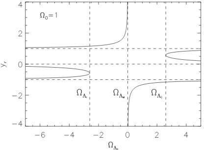
[image:4.595.330.541.172.327.2]illustrated in the Figures (3) and (4), where the root values of f(y)are placed as a function of the cosmological constant for two different values of the density parameter.
[image:4.595.80.286.258.412.2]Figure 3. Real roots off(y)as a function ofΩΛ0, forΩ0= 0.25.
Figure 4. Real roots off(y)as a function ofΩΛ0, forΩ0= 1.
The global properties of the models can be found by con-sidering the behavior of the relation
ΩΛ0 =
(Ω0−1)y−Ω0
y3−y , (21)
which is obtained fromy˙= 0.
The equation (21) has a zero only for Ω > 1 at y = Ω0/(Ω0−1). It also has a local minimum that isΩΛc and
forΩ0>1has a local maximum that isΩΛM. The equation
(21) was sketched in Figure 5 for some values of the density parameter. Comparison with analogous tracings in models
with Λ 6= 0 shows that the branch for y < 1, in the Fig-ures (3) and (4), is not explicitly present in them and for this ΩΛc is not given. This illustrates the difference between the
[image:4.595.79.287.451.604.2]scheme of classifications based on Robertson’s approach and that presented here based on the Glanfield’s work [13].
Figure 5. Plotting the conditiony˙= 0, in the plane (y,ΩΛ0), for different
values of theΩ0parameter that, are indicated in the figure.
The above analysis can be summarized as follows:
A: MODELS WITHΛ<0. They have no particular or crit-ical value for the cosmologcrit-ical constant. They are all well defined, oscillating universes, reaching peaks both closer to 1 the more neative is the cosmological constant. The expan-sion phase always ends fory >1, that is, in our future and so they are physically allowed models. TheΛ = 0 limit is reached smoothly.
B: MODELS WITHΛ>0. Here the scenario is more com-plex. The models may present one or two critical values of the cosmological constant, depending on the value ofΩ0. We
will consider them separately.
MODELS B1: Ω0 ≤ 1. In this case, since we have
ΩΛM ≤ 0, there is only one particular value of the
cosmo-logical constant,ΩΛc. The models with0≤ΩΛ0 ≤ΩΛc are
inflectional and expand indefinitely. The expansion rate de-creases to a minimum and then inde-creases. For large values ofy,y˙=H0Ω1Λ/02y, then the model begins an inflation phase.
However, whenΩΛ0 ≥ΩΛc the expansion starts fromy= 0
and ends wheny <1and, as we will see later, in a finite time. Therefore, these models are not physically allowed, since the universe would never reach the current conditions. There is another possibility, which is to consider the branch starting the expansion in the pointy˙= 0, that is, models without big bang origin. They are monotonous models, type M2 after Robertson. It should be noted that when Ω0 is very small,
models can be produced starting from arbitrarily small val-ues of y, ie quasi-explosive universes. One last possibility is to consider models that begin by contracting to the point
˙
y= 0and then re-expanding.
MODELSB2: Ω0 > 1. In this case, there are two
criti-cal values for the cosmologicriti-cal constant,ΩΛcandΩΛM. The
models withΩΛM <ΩΛ0 <ΩΛc are inflectional. The
toy >1in a finite time (see below) and then collapse. Thus, they are physically allowed. Finally, forΩΛ0≥ΩΛcthe
mod-els are not physically allowed, for the reasons already pointed out.
Thus, models withΩΛ0 ≥ΩΛc are not physically
permit-ted, or do not have a big bang origin. In other words, in the scenario of the big bang type models,ΩΛcis an absolute
up-per bound in the sense that only models withΩΛ0 <ΩΛcare
physically permitted.
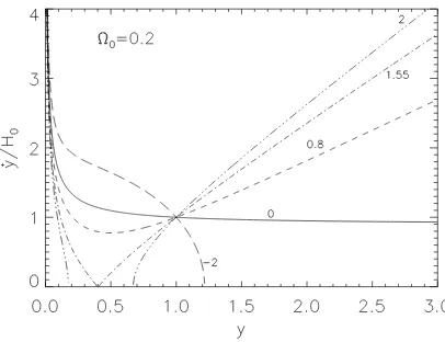
[image:5.595.70.273.252.408.2]The Figure 6 illustrates the different possibilities when we plot the function y(y)˙ for a particular value of the density parameter.
Figure 6. Same as Figure 1, but for models withΛ6= 0, forΩ0= 0.2. The
values ofΩΛ0are indicated in the figure. The valueΩ0= 1.55corresponds
toΩΛ0= ΩΛc
One last comment about Einstein’s static model. Robert-son & Noonan [14] discussed models withΛ6= 0in the plane (λ, µ), where
λ=ΩΛ0
Ω0
e µ=Ω0+ ΩΛ0−1
Ω0
.
The conditionQ3−P2= 0can be written asµ3= (27/4)λ, except forλ= 0, and the static Einstein model corresponds toλE = 1/2, µE = 3/2, which is a particular solution of
this condition. In fact it can be found as a particular case whenΩΛ0andΩ0are the classification parameters. However,
the Einstein case corresponds to the situation where the two parameters are infinite (H0= 0) and the solutions (14 to 16)
can be rewritten as ΩΛc
Ω0 =
ΩΛM
Ω0 =λE=
1 2 e
ΩΛI
Ω0 =−4.
It should be noted, however, that onlyΛE matches with a
critical value of the cosmological constant. The pseudo-ΛE,
defined by the relationΩΛc/Ω0 = 1/2, have no particular
meaning in general, which is in agreement with [13] and [15].
3
Time scale for FLRW models with
Λ
6
= 0
One of the most powerful cosmological tests for models with temporal evolution is undoubtedly the time scale. On
the other hand, it does not contain problems that develop in loop, since the lower limit of the time scale is fixed to the galactic scale, regardless of any cosmological considerations. It is consensual that the strong argument in favor of the expansion hypothesis and the standard model itself are more important than the agreement of the ages of globular swarms with the Hubble constant. Analyzing the situation in de-tail, we will have to conclude that the range of values of H0currently allowed by observational data implies that
non-standard models, in the sense of models withΛ6= 0, can not be put aside.
Time-related problems, which can affect the standard model, are the main argument for a non-zero value of the cosmological constant. Actually, by taking the currently ac-cepted lower values of the age of the older globular swarms (tEG = 1.5×10¹⁰ years [9]), H0 values over 65 Km s−1
Mpc−1 may not be compatible even for the limiting case
Ω0= 0, ifΛ = 0. Since cosmological constant values higher
than this are not excluded by the observations, let us consider models withΛ6= 0that originateH0t0≥1.
First we will calculate the models originating from the big ang. The period of expansion from the big bang to today is obtained by integrating the equation (8),
H0t0=
Z 1
0
r y
Ω0(1−y) + ΩΛ0(y3−y) +y
dy. (22)
It is simple to see that the conditionH0t0>1implies that the
integrating equation (I(y)), can not be monotonous in the in-tegration domain, sinceI(0) = 0andI(1) = 1for any values of the cosmological parameters. Thus, this condition implies thatI(y)has to have a maximum in0≤y≤1. It is simply shown that this maximum occurs forymx= (Ω0/(2ΩΛ0))
1/3.
Forymxbelonging to [0,1] the condition to be imposed is that
ΩΛ0 >Ω0/2. In other words, only models with positive
cos-mological constant and negative deceleration parameter can haveH0t0≥1.
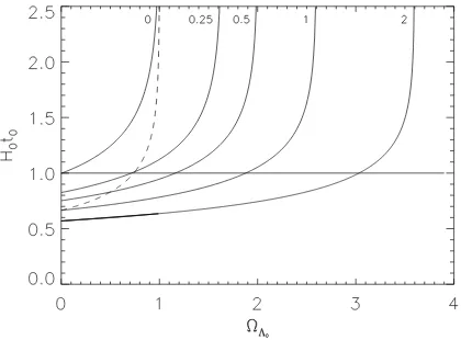
For each model we can calculate H0t0. The results for
0 ≤ ΩΛ0 ≤ ΩΛc are represented in Figure 7. Let us now
comment on some aspects of the figure.
First, we notice that whenΩΛ0= ΩΛc, the time scale is
in-finite. On the other hand, since these cases happen fory <1, these models can never reach the present conditions, so they are not physically allowed. For ΩΛ0 > ΩΛc only models
without big bang are formally allowed. These models are of very small ages, except whenΩΛ0 is very close to ΩΛc.
In principle, both models that are arbitrarily close to the bor-der (ΩΛ0 a little lower or a little upper thanΩΛc) are
phys-ically allowed and can produce arbitrarily large time scales. In addition, as already mentioned before, these models with ΩΛ0 = (1 +ǫ)ΩΛc andΩ0 ≈ 0have initial conditions
arbi-trarily close to those models with big bang. However only the models withΩΛ0= (1−ǫ)ΩΛc(ǫ∼0) have the big bang
origin.
Second, we note that the conditionH0t0≥1is satisfied for
a small range of values of the cosmological constant. This condition determines a particular value of the cosmological constant,ΩΛ1, such that forΩΛ1≤ΩΛ0≤ΩΛc, our condition
as the value of Ω0 increases. On the other hand, only the
values ofΩΛ0 close toΩΛc produce values forH0t0 fairly
greater than 1. Thus, for high values of H0, values ofΩΛ0
[image:6.595.77.287.160.315.2]must be very close to the critical value.
Figure 7. H0t0value as a function ofΩΛ0, for some values of the
den-sity parameter. The numbers in the figure correspond to values ofΩ0.
The dashed line corresponds toH0t0(Ω0,ΩΛ0), for Euclidean models
(Ω0+ ΩΛ0 = 1).
To summarize the results we have shown, we can only say that, with the exception of models close to the boundary, models withΩΛ0 ≥ΩΛc are not physically permitted, either
because they do not meet the conditions as well as because they are not compatible with the ages of globular swarms. If the Hubble constant is greater than 65 Km s−1Mpc−1, we
should consider the conditionH0t0≥1, so, only models with
ΩΛ1 ≤ ΩΛ0 ≤ ΩΛc should be physically acceptable. This
range of values is relatively narrow, as can be seen in Figure 7. For the case of the Euclidean models (Ω0+ ΩΛ0 = 1),
H0t0>1impliesΩΛ0>0.7andΩ0<0.3.
4
Speeds greater than light in a
uni-verse with
Λ
Einstein’s Special Relativity (SR) postulates that the speed of light (c) is an absolute upper bound for all particles. Thus, in a devoid of matter universe (for example, Milne universe), only particles without mass can reach this value. All the others (with mass) have lower speeds. This fact, apparently unimportant, allows us to conclude that time is relative to the observer, that is, a given fact can be observed at different mo-ments by two observers that move with different speeds. With some simple calculations we can affirm that this theory that throws aside the concept of absolute time affirms, on the con-trary, that the time can be dilated and the lengths contracted (in relation to the own rest frame).
General Relativity (GR) encompasses the concepts under-lying SR, but now with the presence of matter. The notion of gravitational force is abandoned. Einstein’s field equations ((3) and
¨ a a =−
4πG
3 (ρ+ 3p) + Λ
3. (23)
tell us how the presence of matter bends or deforms the space in which it is embedded. The coherence of this theory is astounding, having predicted, among other phenomena, the advance of the Mercury perihelion. The light speed remains as an absolute maximum limit, because locally all particles describe trajectories in the space-time, inside their light cone. However, there is a very important feature of our Universe, which results only from observations, which is their expan-sion. In 1929 Edwin P. Hubble [17] noted with surprise that distant galaxies move away from each other at speeds propor-tional to their distance. The proporpropor-tionality parameterHwas called the Hubble ‘constant’, although it is not truly a con-stant, since it varies with the instant of observation (cosmic time)
v=Hd. (24)
This property came to prove that the Universe had a begin-ning.
There is still considerable controversy in the literature about the possibility of higher velocities than light in the Uni-verse. Some authors who argue for the absence of higher recession velocities claim that the expansion of space is a peculiarity of the choice of coordinates made [18], or also that the expansion is locally kinematic [19]. With opposite opinion are authors like Murdoch [20], Harrison [21, 22, 23], Stuckey, [24], Kiang [25, 26, 27] and Davis et. al. [29, 30]. This controversy is no longer recent, as evidenced by the non-acceptance of the expansion of the Universe by Milne, where it proposed an expansion through space, creating a Newto-nian Cosmology [28].
In this work we share the widely held opinion among cos-mologists that the redshift of cosmological origin can not be confused with a Doppler effect. So it seems to us not correct to invoke calculations and aspects of of SR, in a cosmological context, to impose an upper limit equal tocfor cosmological recession velocities. That is why Milne resorts to a solution that is a flat space-time, to oppose the idea of an expansion based on the increase of the scale factor. If the expansion is interpreted as a movement in space, then it is natural that there is a limiting speed. In an expanding universe, in which space is curved by the presence of matter, it is absolutely in-dispensable to distinguish between the speed due only to the expansion (kinematic) of the peculiar speed of an object. In this scenario, objects at rest for a local observer with matter can be seen by sufficiently distant observers at speeds higher than light.
We define a Hubble radius as the distance such that objects at this distance have a recess velocity equal to the light speed (dH = 1/H, we considerc = 1). Objects within the
Hub-ble sphere will have lower velocity and, on the other hand, objects outside the sphere will have a speed greater than that of light. Let’s see what happens to the FLRW models with k= 0.
(i) If we consider Λ = 0, the scale factor has the known forma(t) = αt2/3, whereαis a constant. A galaxy outside our Hubble sphere can thus send us luminous signals that af-ter some time we will be able to pick up. Let us suppose that the galaxy with comoving coordinates (r =re, θ, φ) that in
t = te emits a light signal that will be picked up by us in
t=t0with coordinates (r= 0, θ, φ). The proper distance to
the galaxy from us is given by
dG(t) =a(t)re, (25)
however, the photon being traveling (locally at the speed of light), has a time-varying coordinaterγ(t)and its proper
dis-tance from us will be
dγ(t) =a(t)rγ(t). (26)
We know thatds2= 0for photons, holdingθandφconstants, thendr =±dt/a(t). Integrating this equation, choosing the negative sign because the photon travels in our direction and because we choose the positionr= 0, it comes
Z rγ(t)
re
dr=−
Z t
te
dt′
a(t′) ⇒rγ(t) =re−
3 α
t1/3−t1e/3
.
(27) The galaxy’s comoving coordinate can also be calculated in the same way as the previous
Z re 0
dr=
Z t0
te
dt
a(t) ⇒re= 3 α
t10/3−t1e/3
. (28)
Using the equations (26), (27) and (28) we obtain dγ(t) = 3t0
"
t t0
2/3
−tt
0
#
. (29)
The speed of the photon is easily obtained by deriving the previous equation,
vγ(t) = 3
" 2 3 t0 t
1/3
−1
#
. (30)
The galaxy that emitted the signal is currently at a distance dG(t0) = 3t0
"
1−
te
t0
1/3#
, (31)
supposing that the galaxy emitted its first light signal atte=
0.07t0, it is currently at distancedG(t0)≃1.8t0and its speed
is
vG(t0) = 2
"
1−
te
t0
1/3#
, (32)
that is, vG(t0) ≃ 1.2, so it is almost entering our Hubble
sphere.
As we have seen, the expansion produces significant ef-fects on how matter and radiation can be causally related at distinct points in the Universe. However, it is crucial to know how this expansion is evolving over time, that is, whether it is increasing or decreasing.
In the hypothesis that the expansion rate is decreasing (Universe in deceleration) two scenarios are possible: the Universe expands indefinitely, or after a certain moment it begins to contract giving rise to the Great Implosion (the op-posite of big bang). The latter hypothesis leads to the meeting of all conditions for the formation of a new universe and this scenario perpetuates itself. The cosmological constant is de-cisive in this situation.
(ii) Let us now considerΛ6= 0and see how particles be-have in large-scale. We now be-have to consider the dimension-less scale factor and the differential equation (8) by choosing the positive sign
˙ y=dy
dt =H0
q
Ω0(1/y−1) + ΩΛ0(y
2−1) + 1. (33)
For the flat models (Ω0+ ΩΛ0 = 1), the equation is simplified
dy dt =H0
p
(1−Ω0)y3+ Ω0
√y . (34)
From here, we can integrate the equation
Z √ydy p
(1−Ω0)y3+ Ω0
=H0
Z
dt. (35)
As
Z √ydy p
(1−Ω0)y3+ Ω0
= 2 3
1 √
1−Ω0
sinh−1 r1−Ω0
Ω0 y 3/2
!
,
(36) we can write,
H0
Z t
0
dt′=2
3 1 √
1−Ω0
sinh−1"r1−Ω0
Ω0
y′3/2
#y
0
, (37)
therefore,
H0t=2
3 1 √
1−Ω0
sinh−1
r
1−Ω0
Ω0
y3/2
!
. (38)
In particular fort=t0,
H0t0=
2 3
1 √
1−Ω0
sinh−1 r1−Ω0
Ω0
!
. (39)
The previous expression shows that ifΛ>0, we haveH0t0>
2/3and allows to calculate the age of the Universe. Thus, the scale factor can be obtained explicitly as a function of time
y(t) =
"r
Ω0
1−Ω0
sinh
t3 2H0
p
1−Ω0
#2/3
. (40)
te and since the equation (26) remains valid, we need only
integrate the equation
Z rγ(t)
re
dr=−
Z t
te
dt′
a =−
Z y
ye
dy′
H0a0yy˙
(41) howreis such that
Z re 0
dr=
Z t0
te
dt a =
1 H0a0
Z 1
ye
dy
yy˙. (42) Thus,
dγ(t) = 1
H0
y
Z 1
y
dy′
yy˙, (43)
on the other hand,
H0t0=
Z 1
0
dy ˙
y , (44)
so,
dγ(t) = t0
R1
0
dy
√
Ω0(1/y−1)+ΩΛ0(y2−1)+1
y×
Z 1
y
dy′
yp
Ω0(1/y′−1) + ΩΛ0(y′
2−1) + 1. (45)
Similarly to the above, the photon velocity in this scenario is given by deriving the expression of the photon’s proper distance as a function of time
vγ(t) = ˙arγ(t) +ar˙γ(t) (46)
which leads to
vγ(t) = ˙y 1
H0
Z 1
y
dy′
yy˙ −1, (47)
or yet,
vγ(t) =
q
Ω0(1/y−1) + ΩΛ0(y
2−1) + 1×
Z1
y
dy′
y′p
Ω0(1/y′−1) + ΩΛ0(y′
2−1) + 1−1.(48)
By integrating these equations numerically we can obtain so-lutions for any value of the parameter pair (Ω0,ΩΛ0) with
Ω0+ ΩΛ0= 1. In this way, the Figures 8 and 9 were obtained
for several values of matter density, always for flat models.
5
Horizons
[image:8.595.330.545.364.522.2]Horizon’s concept is familiar to us from everyday experi-ence as the distance to Earth’s surface from which we can not observe. A similar idea happens in Cosmology, but now in re-lation to the distance that light travels in a certain period of time. Because the light speed is the fastest that massless par-ticles can travel, the cosmological horizons provide the limits that our observation can achieve. Just as the horizon on Earth is related to the curvature of this and altitude to which we ob-serve its surface, the cosmological horizons are related to the
[image:8.595.57.297.435.578.2]Figure 8. The Figure illustrates the photon distance is from us from the instant that it was emitted by the galaxy: it initially moves away from us due to expansion, although locally it travels with velocity−1, but also due to expansion the Hubble radius increases, eventually reaching it. From there their distance begins to decrease. In this figure we considered the values (Ω0,ΩΛ0) = (1.0,0.0),(0.3,0.7)and(0.001,0.999)
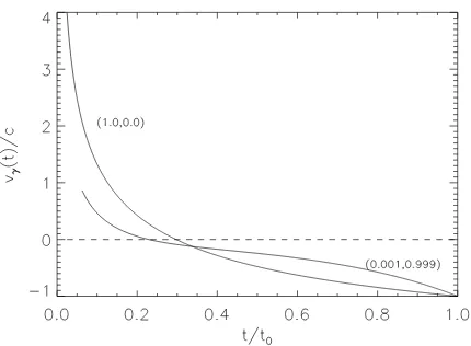
Figure 9. In this Figure we can see that the photon begins by having a speed greater than light moving away from us, but since entering of the Hub-ble sphere, being momentarily ”stopped”, its velocity ends up reaching−1
when it reaches us. In this figure we considered the values (Ω0,ΩΛ0 =
(1.0,0.0))and(0.001,0.999). The values par (0.3,0.7) is very close to the Einstein-de Sitter model(1.0,0.0).
finite value of the light speed and the way the Universe ex-pands. Everything beyond the horizon we say is not causally related to us and no information from these regions can be obtained.
particle horizon1in the instantt0is given by
dhp(t0) =a(t0)
Z t0
0
dt
a(t). (49)
The cosmic microwave background radiation is undoubt-edly the one that was emitted at the longest distance from us It was at this momenttd that there was the decoupling
be-tween matter and radiation. The last scattering surface was emitted at that moment and it is observed by us with a red-shift ofz ≃1000. For higher values of z (consequently for t < td) the Universe was opaque to electromagnetic radiation.
In this sense we can speak in a visual horizon because in fact the microwave background radiation is the most distant in-formation we can get. Let us calculate, at what distance this radiation was from us at the instant it was emitted, to the flat model without cosmological constant (Ω0= 1)
d(td) =a(td)
Zt0
td
dt
a(t)⇒d(td) = 3td
"
t0
td
1/3
−1
#
.
(50) As the red-shift is related to the scale factor by the relation z=a(t0)/a(td)−1, using the scale factor expression we can
write
d(td) = 3td
√
z+ 1−1
. (51)
By the Hubble law, the speed at that moment would be v(td) =H(td)d(td) = 2
√
z+ 1−1
, (52)
since for this modelHt= 2/3. Thus, at the instant the radia-tion was emitted, that matter traveled at a speedv(td)≃61.3.
Also we can know the speed that currently has this matter
d(t0) = 3t0
"
1−
td
t0
1/3#
= 3t0
1−√1 z+ 1
. (53)
The current speed is
v(t0) = 2
1−√ 1 z+ 1
, (54)
that is,v(t0)≃1.94. However, there is something that we can
not observe and that is still more distant. The furthest matter is currently traveling at2(z→ ∞), (on the particle horizon), but locally it is at rest for a local observer.
Now let us consider the more general case. Let us base ourselves on the equation (49) now with the form
d(t0) =
Z 1
0
dt
y2H, (55)
where y = a(t)/a0 e H(y) = pΩ0/y3+ ΩΛ0+ Ωk0/y2.
Initially and for simplicity we will consider the flat model (Ωk0 = 0) with the two extreme cases: Ω0 = 1andΩ0 = 0.
In this case we have respectively H(y) = H0y−3/2 and 1Generally, the proper distance to the particle horizon at the instanttis
given bydhp(t) =
Rr′
0
√g
rrdr.
H(y) =H0, for each case. From here it comes that
Ω0= 1 ⇒ dhp(t0) =
Z 1
0
dy y2H
0y−3/2
= 1 H0
Z 1
0
y−1/2dy= 2 c
H0 (56)
Ω0= 0 ⇒ dhp(t0) =
Z 1
0
dy y2H 0
= 2 1 H0
−1 + 1 0+
= +∞, (57)
that is, as we have already seen above, there is a particle hori-zon for the matter dominated flat model, but we now see that there is no particle horizon for the vacuum dominated flat universe. It is time to consider the most general possible situ-ation usingH(y)replacing the equationΩ0+ ΩΛ0+ Ωk0= 1
in this, we obtain the following equation to integrate
dhp(t0) = H1 0
Z 1
0
dy
p
Ω0(y−y2) + ΩΛ0(y4−y2) +y2
. (58)
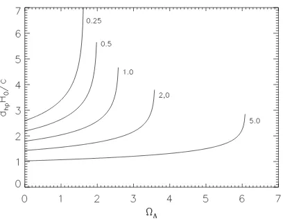
This equation can be integrated numerically for many val-ues of the density parameters. In Figure 10 we setΩ0 and
integrated the equation in function ofΩΛ0. We found that for
each value ofΩ0 there is a value ofΩΛ0 for which there is
no horizon. But this fact is intrinsically related to the asymp-totic values obtained also in Figure 7. In the particular case ofΩ0= 0being free the two other parameters, only obeying
the relationΩΛ0+ Ωk0 = 1, the proper distance has the form
dhp(t0) = H1 0
Z 1
0
dy
p
ΩΛ0(y4−y2) +y2
, (59)
asΩΛ0(y
4−y2)+y2≥0we see that there are two solutions:
y2= 0ouy2=ΩΛ0−1
ΩΛ0 , but the second solution will only give
real values ofyify2≥0⇒ΩΛ0 >1. But in this hypothesis
the allowed interval fory is y ∈
r
ΩΛ0−1 ΩΛ0 ,1
, that is, an integration between 0 and 1 can not be made. Thus, in the case of Ω0 = 0 we must haveΩΛ0 ≤ 1. In this case the
integration will be
dhp(t0) =−p 1
1−ΩΛ0
×
"
ln −2ΩΛ0−1−
p
1−ΩΛ0
p
ΩΛ0y2−ΩΛ0+ 1
y
!#1
0
=−p 1
1−ΩΛ0
×
n
lnh−2ΩΛ0−1−
p
1−ΩΛ0
i
−ln(−2×0)o
= +∞, (60)
Figure 10. Proper distance to the particle horizon for several values ofΩ0
(indicated) as a function ofΩΛ0.
6
Conclusions
We have shown that the classification scheme for the case ofΛ 6= 0which is usually presented is not complete, as al-ready predicted by Glanfield [13]. ForΛ<0, the results are the same as the old work of Robertson [11]. But for models with positive values of the cosmological constant, we con-clude that depending on the value of the density parameter, there are one or two particular values of ΩΛ0 that separate
the different types of models,ΩΛM andΩΛc(ΩΛc >1), with
ΩΛM <ΩΛcandΩΛM ≥0only whenΩ0>1.
The models withΩΛ0 <ΩΛM (orΩΛ0 <0whenΩΛM is
negative) are oscillating independent of the curvature param-eter. The end of the expansion phase occurs fory > 1, so these are physically allowed models.
WhenΩΛM is positive, the models with ΩΛM < ΩΛ0 <
ΩΛc are inflectional. The expansion never ends and start an
inflationary phase for large values ofy.
Finally, the models withΩΛ0 >ΩΛcare oscillating if they
start at y = 0. Otherwise, they are inflectional. The for-mer are not physically permitted since the expansion phase never reaches the present conditions,y= 1. The others start fromy > 0, in addition to losing the advantages of the big bang origin, usually produce a reduced time scale. Formally the boundary models with ΩΛ0 = (1 +ǫ)ΩΛc (ǫ ∼ 0) can
produce sufficiently large time scales, but only for values of ΩΛ0virtually indistinguishable fromΩΛc. In this context, we
have already mentioned that for very low values of the den-sity parameter, this kind of models may even have an origin of almost big bang. However, such solutions have only a the-oretical interest, since they are physically equivalent to the singular casesΩΛ0 = ΩΛc and, if we want a start with big
bang we haveΩ0= 0andΩΛc= 1.
We can thus conclude that the models withΩΛ0 ≥ΩΛcare
excluded.
In the case whereH0 is greater than 65 Km s−1Mpc−1,
the time scales for the models withΛ = 0 are very small compared to the lower of globular swarms ages estimates. The conditionH0t0 >1will have to be imposed. The
con-sequence is that only values of ΩΛ0 very close to the
crit-ical value are allowed. For the Euclidean case (k = 0), 0.74≤ΩΛ0 ≤1.
We also concluded that the effect of the expansion of the Universe produces the effect of particles (with mass or mass-less) being able to overcome the light speed barrier, when observed in large scale. Recent observations in supernovae seem to leave no doubt among researchers that the Universe is in accelerated expanding. These conclusions are contrary to the convictions of most cosmologists and the presence of the positive cosmological constant solves this question. This implies that the expansion of the Universe is unique and not reversible, which causes that the own life of the stars, after sufficient time, is extinguished.
All of these models have particle horizons except for point values of the parameters (Ω0,ΩΛ0), or whenΩ0= 0. For all
models there is no event horizon.
REFERENCES
[1] W. Rindler. Essential Relativity. Heidelberg: Springer,
(1977).
[2] S. Perlmutter et al. Nature, 391:51, (1998).
[3] A. G. Riess, et al. Astron. Journ., 116:1009, (1998).
[4] A. G. Riess et al. Astron. J., 116:1009, (1998).
[5] A. A. Starobinsky. Phys. Lett., 91B:99, (1980).
[6] A. H. Guth. Phys. Rev. D, 23:347, (1981).
[7] A. Albrecht, P. J. Steinhardt. Phys. Rev. Lett., 48:1220, (1982).
[8] A. Linde. “Quantum cosmology and the structure of inflation-ary universe”. gr-qc/9508019, (1995).
[9] A. R. Sandage. ARA&A, 26:561, (1988).
[10] J. R. Primack. “Cosmological Parameters”.
astro-ph/0007187, (2000).
[11] H. P. Robertson. Rev. Mod. Phys., 5:62, (1933).
[12] R. Stabell, S. Refsdal. MNRAS, 132:379, (1966).
[13] J. R. Glanfield. MNRAS, 131:271, (1966).
[14] H. P. Robertson, T. H. Noonan. Relativity and Cosmology. Philadelphia: W. B. Saunders, (1968).
[15] J. E. Felten, R. Isaacman. Rev. Mod. Phys., 58:689, (1986).
[16] W. H. Press, B. P. Flannery, S. A. Teukolsky, & W. T. Vetter-ling. Numerical Recipes. Cambridge: Cambridge Univ. Press, (1986).
[18] Don Page. “No Superluminal Expansion of the Universe”.
gr-qc/9303008, (1993).
[19] J. A. Peacock. Cosmological Physics. Cambridge University Press, (1999).
[20] H. S. Murdoch. Q. J. R. Astr. Soc., 18:242, (1977).
[21] E. Harrison. Cosmology. Cambridge University Press, (1981).
[22] E. Harrison. Ap. J., 383:60, (1991).
[23] E. Harrison. Ap. J., 403:28, (1993).
[24] W. M. Stuckey. Am. J. Phys., 60(2):142, (1992).
[25] T. Kiang. Chin. Astron. Astrophys., 21:1, (1997).
[26] T. Kiang. “Can We Observe Galaxies that Recede Faster than Light ? – A More Clear-Cut Answer”. astro-ph/0305518, (2003).
[27] T. Kiang. “Time, Distance, Velocity, Redshift: a personal guided tour”. astro-ph/0308010, (2003).
[28] E. A. Milne. Q. J. Math. Oxford, 5:64, (1934).
[29] Tamara M. Davis, Charles H. Lineweaver. “Superluminal Re-cession Velocities”. astro-ph/0011070, (2001).
[30] Tamara M. Davis, Charles H. Lineweaver, John K. Webb. Am.