An algorithm to identify vibration modes of PCB using free response data

Journal of Chemical and Pharmaceutical Research, 2013, 5(9):291-297

Research Article

_{CODEN(USA) : JCPRC5}

ISSN : 0975-7384

An algorithm to identify vibration modes of PCB using free response data

Dapeng Zhu

School of Traffic and Transportation, Lanzhou Jiaotong University, Lanzhou, China

_____________________________________________________________________________________________

ABSTRACT

Researches on the dynamic properties and vibration modes identification of Printed Circuit Board(PCB)loaded on train are important for the train safety in transportation. In this paper, a novel approach to identify the vibration modes of PCB is presented. The free acceleration response of the PCB is expressed as the sum of linear exponentials, the zeros and residues of the free response are identified by the Prony method, the zeros and residues are optimized by the nonlinear total least 1-norm method. An experiment system is formulated to record the free response of PCB, the zeros and residues are identified and optimized, the simulation results indicate the approach presented in this paper is accurate to identify the PCB vibration modes. The algorithm presented in this paper is more robust and more accurate to identify PCB vibration modes. The technique in this paper is useful for PCB design and the safety management of train.

Key words: PCB vibration modes, Prony method, Nonlinear total least norm method, Free response data

_____________________________________________________________________________________________

INTRODUCTION

Nowadays, more and more electronic equipments are installed on the train to ensure the safety, efficiency, economy of train transportation. Thus, the dynamic properties modeling and vibration modes identification of PCB in the electronic equipments are important for optimal design of PCB, the safety of train transportation, and the proper train equipment management.

Alsaleem et al. [1] presented an investigation into the effect of the motion of PCB on the response of MEMS system to shock loads. A two-degrees-of-freedom model is used to model the motion of the PCB and the microstructure. Y.S. Chen et al. [2] developed a methodology which combines the vibration failure test, finite element analysis (FEA), and theoretical formulation for the calculation of the electronic components fatigue life under vibration loading. H. William and J. Ping[3] formulated several mathematical models for determining the optimal sequence of component placements and assignment of component types of PCB, a hybrid genetic algorithm was adopted to solve the models. Pitarresi[4] presented PCB modeling technique under random vibration technique, the model presented by the authors can be used to predict the fatigue life of the PCBs. A PCB plane model is proposed by Beak et al.[5], the model reflects two frequency-dependent losses, namely, skin and dielectric losses, with the proposed model, not only ac analysis but also transient analysis can be easily done for circuits including various non-linear/linear devices. Labarre et al.[6] describes a method for modeling the PCB employed in high-frequency (range 10 kHz-1 MHz), medium-power (several kW) static converters, in order to simulated their conducted interference emissions.

______________________________________________________________________________

FREE RESPONSE OF PCB

Assuming PCB as a lightly damped structure, one can model the free acceleration response of the system as



ie t

A t

x i i

1 2 ) 1 sin( ) (     

 (1)

where M is the number of the vibration mode in the system, ζi is damping ratio of ith mode, ωi is undamped angular

frequency of the ith mode, =2πfi, where fi is the undamped natural frequency in Hertz, φi is the phase delay of the ith

mode in radians, and Ai is the amplitude of the ith mode. If the free response of the system is sampled every ΔT

seconds, then (1) can be rewritten as



ie n T

A T n

x i i

1 2 ) 1 sin( ) (     

 (2)

Expanding (2) in complex exponential form gives

N n z B y B y B y B A A T n x M i n i i M i T n i i T n i i M i T n i i M

i i T Tn

n T T i i i i i i i i i i i , , 2 , 1 e e j 2 e e j 2 ) ( 2 1 2 1 2 2 1 1 2 1 2

1 -j ( j 1 )

) 1 j ( j 2 2                                    









From (3), each vibration mode yields two complex exponentials. The complex amplitudes are

i i

i i i

i A B A

B  2 j

j 1

2 ( /2j)e ( /2j)e



    (4)

The complex exponentials corresponding to these amplitudes are

2

2 _{j 1}

2 1

j 1

2 e e

i i i i i i i i i i y

y        (5)

and T p T i i i e y

z     (6)

From (2), one can see that the acceleration free response of the mechanical system can be expressed as the linear sum of the complex exponentials. In (3), zi is called system zeros and Bi is called the residues, in (6), pi is called

system poles.

IDENTIFY ZEROS AND RESIDUES USING PRONY METHOD

Since Prony method is a technique for modeling the sampled free acceleration response of the system as a sum of a finite number of exponential terms, the zeros and residues of the sampled data in (3) can be identified by Prony method. This algorithm can be summarized as follows.

Step 1: Record the free acceleration response data of PCB: x[1],x[2],…x[N], let pe>>2M, compute matrix R given

by              ) , ( ) 1 , ( ) 0 , ( ) , 2 ( ) 1 , 2 ( ) 0 , 2 ( ) , 1 ( ) 1 , 1 ( ) 0 , 1 ( e e e e e e p p r p r p r p r r r p r r r       

R (7)



Determine the effective rank 2M of matrix R and the AR coefficients a1,a2,…,a2M by use of SVD-TLS method[7];

Step 2: Form the polynomial

0

1 2

2 1

1   

  M

Mz a z

a  (8)

and solve to find the roots which are the system poles zi in the series of complex exponentials in (3);

Step 3: Rewrite (3) as matrix form:

x ZB

Where              N M N N M M z z z z z z z z z 2 2 1 2 2 2 2 2 1 2 2 1        Z ,              M B B B 2 2 1  B ,              ) ( ) 2 ( ) 1 ( N x x x          x

Because N>2M, then, vector B can be obtained by

x Z Z] [Z

B T 1 T (9)

Where the superscript T and -1 denote the transpose and inverse operation of the matrix respectively.

Using the steps outlined above, one can obtain the number of the vibration mode terms 2M, the system zeros zi and

residues B.

OPTIMIZE SYSTEM ZEROS AND RESIDUES BY NONLINEAR TOTAL LEAST NORM METHOD

The identification accuracy of system zeros and residues is affected by many factors: First of all, the measurement noise may make the identification inaccurate, both in terms of variance and bias. Secondly, if some vibration mode of PCB is too weak, or polluted by noise, the identification results will also be deviated from the real value. Moreover, it is difficult to determine the exact time at which the free response of the mechanical system begins, which also make Prony method inaccurate. Thus, it is necessary to optimize the signal zeros zProny and residues BProny identified by the Prony method.

Equation (3) can be rewritten in matrix form

                                        ) ( ) 2 ( ) ( 2 2 1 2 2 1 2 2 2 2 2 1 2 2 1 T N x T x T x B B B z z z z z z z z z M N M N N M M                (10)

Or in abbreviated form

Q(z)B=x (11)

Where z=[z1, z2, …, z2M]. In (10), an over determined nonlinear system is formulated. To obtain the approximate solution to this system, where errors may occur in both the vector x and in elements of the Q(N×2M), where N>2M, the parametric problem can be stated as the following minimization problem

p z z B z r B z ˆ ) , ( min

,  (12)

______________________________________________________________________________

The computational results[8,9] show clearly the benefit of using the 1-norm, and its robust performance when data includes some larger errors. Specifically, the errors in the approximation obtained by the 1-norm algorithm are independent of the set of largest errors in the data vector x, and dependent primarily on the set of smallest errors in the data vector x. This is contrast to any method which minimizes the residue in the 2-norm or 1-norm, where the errors in the approximation are proportional to the set of largest errors in vector x. Thus, in this paper, we choose

p=1.

Compute the minimum solution to (12) iteratively by linearizing the residue r(z,B)

r(z+△z,B+△B)=r(z,B)-Q(z)△B-J(z,B)△z (13)

Where J(z,B) is the Jacobin, with respect to z, of Q(z)B. Let zj represent the jth column of Q(z), then one can obtain

J(z,B) by

   

 

   

 

      

 

 



M N

M N

N

M M

M j

M j

j

C Nz C Nz C Nz

C z C

z C z

C C

C

z z B

2 1 2 2 1 2 1 1 1

2 2 2

2 1 1

2 2

1 2

1

2 2

2 )

( ) , (

    

 

z B z Q B z J

(14)

Then, the signal zeros z and residues B can be optimized by the following steps:

Step 1: Set the initial value of the iteration: z=zProny, B=BProny, zˆzProny, where zProny and BProny are signal zeros and

residues vectors identified by modified Prony method discussed in section 3, zˆ is the estimation of the signal zeros

vector. Formulate matrix J(z,B) and Q(z) according to (14) and (11) respectively.

Step 2: Solve the minimization problem as follows

1 1

, ₍ˆ ₎ min

) , ( ) (

min Gu h

z z

r Δz

ΔB 0 0

B z J z Q

u ΔB

Δz _  

   

           





(15)

Where

      

Δz ΔB

u ， _

  

  

0 0

B z J z Q

G ( ) ( , ) ， _

    

 

) ˆ (z z r h

Solve this minimization problem, one can obtain vector u.

Step 3: Set z=z+Δz,B=B+ΔB, zˆz, compute J(z,B) and Q(z) by (14) and (11), compute residue r by r=x-Q(z)B.

Repeat step 2 and step 3, until ||z||1 and ||B||1 is less than the set tolerance value or they vary little in the successive iterations.

In Step 2, the minimization problem can be solved as a linear program, to illustrate this, the linear program for p=1 is summarized as follows.

Introducing the scalars σi (1≤i≤2M+N), representing the absolute values of the components of vector Gu-h, the

corresponding linear program is given by

   

   





i i i i N M

i i u _i

σ h u g σ T 2

1 ,

subject to min 

 (16)

Where giT is the ith row of matrix G, hi is the ith row of matrix h, let σ=[-σ1,-σ2,…, -σ2M+N]T≤0. Then (16)

    

                 

 

 

 

h h σ u I G

I G σ e

σ u,

N M

N M N

M

2 2 T

2

subject to max

(17)

Where T

2MN

e is a column vector, all elements in this vector are 1. We consider this to be a dual linear program, and solve the equivalent primal

     

 

               



 



 



0 y y y

y

I I

G G y h y h

y , y

2 1 2

2 1 2 2

T T 2 T 1 T

, , 0 subject to

) (

min

2 1

N M N

M N

M e

(18)

The optimal solution to (18) will give the optimal dual vectors u and σ, by choosing the scalars σi

sufficiently large, a feasible solution to the dual problem (17) is always obtained. The dual is also bounded since eT2MNσ0. Therefore, both the dual and the primal have optimal solutions.

The nonlinear total least 1-norm method is a nonlinear iterative algorithm. It’s important to find a proper start point of the iterations. In this paper, we choose the zeros and residues identified by the modified Prony method zprony and Bprony as the start point of the iterations. Because zprony and Bprony are near enough to the true zeros and residues, the optimal results can be obtained by the nonlinear total least 1-norm algorithm.

EXPERIMENTAL DATA AND ANALYSIS

The experiment system is schematically shown in Figure 1, PCB is bolted with the vibration table. In present work, a data acquisition system is used to obtain the acceleration data of the excitation and response of the system. The data acquisition system is made up of five parts: two piezoelectric accelerometers, low-pass anti-aliasing filter, charge amplifier, the dynamic data acquisition equipment and computer. All the data collection process in this work was under the control of the YE7600software package.

Vibration controller

Low-pass filter Charge amplifier

Dynamic data acquisition equipment Vibration table

Computer Accelerometer

Time Half-sine excitation PCB

Bolt

Fig.1 The experimental configuration

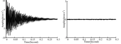
In this paper, a half-sine excitation is generated from the vibration table, and exerted on PCB. According to the field test results[10], the time duration of the excitation is set to be 30ms, the altitude of the excitation is set to be 120m/s2. The acceleration response of the PCB is recorded by the data acquisition system, the time when the vibration table excitation ends can be regarded as the starting time instant of the free response of PCB. The free acceleration response data of PCB is shown in Figure 2(a). The Prony method is carried out. The four vibration modes corresponding to 8 complex system zeros zProny and residues BProny are estimated and shown in Table 1. zProny and

BProny are optimized by use of the nonlinear total least 1-norm method discussed in section 4, after several iterations,

the accurate estimation of the system zeros z and residues B are shown in Table 1. Substitute optimized zeros and residues in Table 1 into (3), one can obtain the predicted vibration signal. The difference between the original signal and the predicted signal is shown Figure 2(b).

0 0.05 0.1 0.15 0.2 0.25 0.3 -10

-5 0 5 10

Time(Second)

A

m

p

li

tu

d

e

(m

/s

2)

(a)

0 0.05 0.1 0.15 0.2 0.25 0.3 -5

0 5

Time(Second)

A

m

p

li

tu

d

e

(m

/s

2)

(b)

______________________________________________________________________________

Once the optimized system zeros z and residues B are obtained, the parameters of each vibration mode can be obtained by

1 2

2 

 i

i B

A iactan(imag(B2i1)/real(B2i1))-π/2

where imag and real denote the imaginary and real part of the complex value. Let

T) 2π /( | |

ln 2 1 

 

 _{i i i}

i f z

p 

T) ))/(2π )/real(

( actan(imag

1 2 1 2 1

2 _{ }



 i i i i

i f z z

q  therefore

2 2

i i

i p q

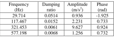
f   i 1(qi/ fi)2

According equations above, the vibration modes parameters corresponding to the system zeros and residues in Table 1 can be obtained and shown in Table 2.

Table 1. Zeros and residues identification results of PCB free response data

Modes zProny BProny z B Mode 1 0.984

±0.038i

-0.476 ±0.110i

0.997 ±0.037i

-0.445 ±0.146i Mode 2 0.984

±0.157i

0.885 ±0.735i

0.987 ±0.147i

0.863 ±0.707i Mode 3 _±0.393i 0.917 _±1.148i 4.328 _±0.392i 0.917 _±1.159i 4.672

Mode 4 0.745 ±0.660i

0.668 ±0.143i

0.740 ±0.647i

0.624 ±0.171i

Table 2. Vibration modes parameters estimation results

Frequency (Hz)

Damping ratio

Amplitude (m/s2₎

Phase (rad) 29.714 0.0514 0.936 -1.925 117.467 0.0152 2.231 0.733 321.453 0.0061 9.627 0.924 577.198 0.0068 1.256 0.732

CONCLUSION

Because of its complex structure, Printed Circuit Board(PCB) usually has multiple vibration modes. The free acceleration response of the PCB can be expressed as the linear combination of complex exponentials, the residues and zeros of PCB can be obtained by the use of Prony method. However, the Prony accuracy of Prony method is affected greatly by the noise in the recorded data, moreover, the weak vibration modes in the PCB free response data can not be identified accurately by Prony method as well. Therefore, in present work, a iterative algorithm, called nonlinear total least 1-norm method is adopted to optimize the identification results. The simulation results indicates the approach incorporates the Prony method with the nonlinear total least 1-norm method presented in this work is accurate. The vibration mode parameters can be used to learn the nature of PCB, to assess the security of PCB in the transportation environment, and they are very important for the PCB design, reliability assessment and structure improvement.

Acknowledgements

This research is sponsored by Basic Scientific Research Special Fund of Gansu Institution of Higher Education, and the author is grateful to the technique assistance from transportation lab in School of traffic and transportation, Lanzhou Jiaotong University.

REFERENCES

[1]Alsaleem F., Younis M.I., Miles R., 2008. Journal of Electronic Packaging,130:31002-31012. [2]Chen Y.S., Wanga C.S., Yanga Y.J., 2008. Microelectronics Reliability, 48:638-644.

[3]William H., Ping J., 2009. Expert Systems with Applications, 36:7002-7010.

[5]Beak J., Jeong Y., Kim S., 2004. IEICE Transactions on Electronics, E87C:1388-1394. [6]Labarre C., Petit Ph., et al., 1998. The European physical journal, 3:169-181.

[7]Huffel S.V., Cheng C.L., et al., 2007. Computational Statistics and Data Analysis, 52:1076-1079. [8]Rosen J.B., Park H. and Glick J., 2000. Optimization and Engineering, 1: 51-65.