NSL
Research Report RR-1
Local-Area
Internetworks:
Measurements
and Analysis
Glenn Trewitt
networks. NSL also offers training and consulting for other groups within Digital.
NSL is also a focal point for operating Digital’s internal IP research network (CRAnet) and the DECWRL gateway. Ongoing experience with practical network operations provides an important basis for research on network management. NSL’s involvement with network operations also provides a test bed for new tools and network components.
We publish the results of our work in a variety of journals, conferences, research reports, and technical notes. This document is a research report. Research reports are normally accounts of completed research and may include material from earlier technical notes. We use technical notes for rapid distribution of technical material; usually this represents research in progress.
Research reports and technical notes may be ordered from us. You may mail your order to:
Technical Report Distribution Digital Equipment Corporation
Network Systems Laboratory - WRL-1 250 University Avenue
Palo Alto, California 94301 USA
Reports and notes may also be ordered by electronic mail. Use one of the following addresses:
Digital E-net: DECWRL::NSL-TECHREPORTS
Internet: [email protected]
UUCP: decwrl!nsl-techreports
To obtain more details on ordering by electronic mail, send a message to one of these
addresses with the word ‘‘help’’ in the Subject line; you will receive detailed
Local-Area Internetworks:
Measurements and Analysis
Glenn Trewitt
March, 1990
Abstract
The effectiveness of a local-area internetwork is evident in its
to-end performance and reliability. The dominant factors limiting to-
end-to-end performance are router delay and the ‘‘fit’’ of traffic patterns to
the topology. Internetwork reliability may be enhanced by
conser-vative topological design, even in the face of unreliable network or
router technology. These issues are crucial to network design.
This dissertation describes the results of studying the Stanford
Univer-sity Network, a large internetwork consisting of interconnected,
local-area networks. To prove this thesis, I made measurements of router
delay, local traffic characteristics, network topology, and traffic
pat-terns in the Stanford internet.
This report reproduces a dissertation submitted to the Department of
Electrical Engineering and the Committee on Graduate Studies of
Stanford University in partial fulfillment of the requirements for the
degree of Doctor of Philosophy.
Copyright
1993 Digital Equipment Corporation
I would like to thank John Hennessy, my advisor, for his support for this research and
his patience with the many detours I’ve taken along the way.
David Boggs, my second reader, gave countless suggestions that made the prose and
figures more direct and clear. His emphasis on directness and clarity helped focus the
research as well.
This research would not have been possible without the equipment, encouragement, and
conference admissions provided by the Networking Systems group at Stanford. Bill
Yundt, Ron Roberts, and Jim Powell were notably helpful. Closer to home, I owe
Charlie Orgish a tremendous debt for being ready to provide help and equipment on
short notice.
My computing environment was greatly enriched by the tools provided by Mark Linton’s
InterViews project here at Stanford. John Vlissides and John Interrante’s idraw program
made drawing the figures a pleasant task.
Craig Partridge’s partnership with me in network management standards activities helped
shape many of my ideas about the tools and methods required for network
manage-ment. This “distraction” provided me with many helpful contacts in the “real world” of
networking.
Lia Adams, Harold Ossher, and John Wakerly were always ready to listen to my ideas
and provide suggestions and encouragement. The many friends in my church and choir
my life.
The research reported in this dissertation was supported by the Stanford Computer
Sys-tems Laboratory.
Abstract i
Acknowledgments v
1 Introduction 1
1.1 Local-Area Internetworks 2
1.2 Wide-Area Internetworks 3
1.3 Model and Terminology 4
1.4 Model of Internetworking 9
1.4.1 Internetwork Maps 9
1.5 Synopsis 12
2 Router Delay 14
2.1 Why are Internetworks Slow? 14
2.1.1 Speed-of-Light Delay 15
2.1.2 Link Bandwidth 16
2.1.5 Routing Delay 18
2.1.6 Network Bottlenecks — Congestion 19
2.1.7 So What Can We Control? 19
2.1.8 End-to-End Delay Variance 21
2.2 Factors Affecting Router Performance 22
2.2.1 Environmental Factors 23
2.2.2 Case Studies 24
2.3 Queuing Network Model of a Router 25
2.3.1 Results of the Simple Model 26
2.3.2 A More Complete Model 27
2.4 Router Measurements 29
2.4.1 Measurement Results 32
2.5 Reconciling the Measurements and the Model 35
2.5.1 Scheduling Delay 36
2.5.2 Ethernet Contention 37
2.5.3 Controlled Workload Experiments 37
2.5.4 Arrival Time Distribution 39
2.5.5 Using Simulation to Measure Burstiness 42
2.6.1 Results with Cache Enabled 46
2.6.2 Results with Cache Disabled 48
2.7 Conclusions 49
2.8 Future Measurement Work 51
3 Internet Topology 53
3.0.1 Common Sense and Assumptions 54
3.1 Measures of a Topology 55
3.2 Internetworks With No Redundancy 56
3.3 Measuring Robustness 60
3.3.1 Partition Fraction 62
3.4 Failure Set Trimming 65
3.5 Double Faults 65
3.6 Measurements of the Stanford Internetwork 68
3.6.1 Stanford Networking Environment and Evolution 68
3.6.2 Redundancy Results 74
3.6.3 Partition Fraction Results — Single Faults 75
3.6.4 Partition Fraction Results — Double Faults 77
3.6.5 Summary of Analysis 80
4 Traffic Patterns 82
4.1 Measurement Technology and Methodology 83
4.1.1 Interface Statistics 84
4.1.2 Routing Table 85
4.1.3 Bridge Statistics 87
4.2 Network Map Annotated With Traffic Volume 88
4.3 Routing Matrix 90
4.3.1 Other Ways to Collect Routing Data 94
4.4 Conclusions 96
5 Conclusions 97
5.1 Future Work 99
5.2 Network Monitoring Lessons 101
5.2.1 Data Gathering 101
5.2.2 Data Processing and Storage 103
5.2.3 Data Presentation 104
Bibliography 106
1.1 Hierarchy of Network Objects 7
2.1 Two Sample Internets 20
2.2 Breakdown of End-to-End Delay 20
2.3 Router Characteristics 24
2.4 Summary of Router Analysis 50
3.1 Analysis of Topology in Figure 1.2 64
4.1 Networks With Heavy Internet Loads 90
1.1 Simple Topology Schematic 10
1.2 Simple Topology Map 10
1.3 Topology Schematic With Bridges 11
1.4 Topology Map With Bridges 11
1.5 Topology Map Showing Traffic Levels 11
2.1 Simple Queuing Network Model 25
2.2 Excerpt of Process Statistics 26
2.3 Delay and Number in System vs. Offered Load 27
2.4 More Realistic Queuing Network Model 29
2.5 Router Measurement Setup 33
2.6 Delay Measurements — 2 Sec Samples 34
2.7 Delay Measurements — 1 and 4 Sec Samples 34
2.8 Delay vs. Offered Load, Worst Case 36
2.9 Delay vs. Rate and Size for Isolated Router 38
2.12 Simulation Algorithm 41
2.13 Simulated and Actual Delay vs. Arrival Rate 41
2.14 Original and Modified Simulation vs. Actual Delay 43
2.15 Average Packet Size vs. Time 44
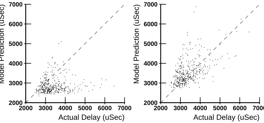
2.16 Original and Modified Model Prediction vs. Actual Delay 45
2.17 Simple Model and Modified Model Results 47
2.18 Simple Model and Modified Simulation Results 49
3.1 Decomposition of Example Topology 57
3.2 vs. for Varying Interfaces 58
3.3 Sample Internet and Two Possible Improvements 60
3.4 Two Sample Topologies 63
3.5 An Independent Fault Pair 67
3.6 A Dependent Fault Pair 67
3.7 Stanford University Network of Aug 6, 1986 71
3.8 Stanford University Network of Nov 10, 1987 72
3.9 Stanford University Network of Apr 29, 1988 73
3.10 Trace of for Stanford Internet 75
3.11 for Ten Worst Single Faults vs. Time 76
4.1 Statistics for One Router Interface 84
4.2 Excerpt from Routing Table 86
4.3 Statistics for One Bridge Interface 87
4.4 Stanford Network with Traffic Volumes 89
4.5 Traffic Source-Destination Matrix 92
4.6 Cumulative Traffic Distribution 94
Introduction
This dissertation argues that router delay and topology are the two key points of local-area
internetwork design. End users perceive two aspects of network performance: speed and
availability. Speed is evident in the network as the end-to-end packet delay or as data
throughput. Delay through routers is the major component of end-to-end delay. Network
availability (“can I get from here to there, now”) may be enhanced by conservative
topological design, even if router or network technology is failure-prone. These two
factors, more than anything else, determine the end user’s perceptions of how “good” the
network is.
This dissertation describes the results of studying the Stanford University Network, a
large internetwork consisting of interconnected, high-bandwidth, local-area networks. To
prove the above thesis, I made the following measurements:
Router delay was measured, noninvasively, for all traffic through the router.
Al-though the end-user perceives end-to-end delay, it is difficult to measure end-to-end
delay for all types of traffic, since instrumentation can’t monitor all traffic in the
internet simultaneously.
Local traffic characteristics, such as packet sizes and interarrival times.
Topological characteristics of the internetwork, such as redundancy and robustness.
Traffic patterns through the internetwork.
Many of the tools developed for this research turned out to be valuable network
manage-ment tools, and continue to be used by the Networking Systems group at Stanford for
day-to-day management of the internetwork.
1.1
Local-Area Internetworks
Local-area networks (LANs) are increasingly popular. Even the smallest workstations
may have a network interface, and many rely on a network for essential services such
as file transfer and mail. Ethernet (10 MBit/Sec) is currently the dominant technology
used at Stanford1; parts of the network will soon be upgraded to optical fiber technology
(100 MBit/Sec FDDI). One common characteristic of local-area networks is that they are
limited in size, both in the number of nodes that may be connected and in their maximum
physical size. The high speed and low delay characteristics of LANs are a direct result
of their limited size.
The solution to this size limitation is to connect LANs together into a local-area
in-ternetwork. The connections between networks can be made with either routers (often
referred to as gateways) or bridges. The choice between the two has been the topic of
heated debate in networking circles, and both have valid applications. For the purposes
of this dissertation, they are equivalent — they both selectively forward packets from one
network to another and take a non-zero amount of time to process each packet. In this
dissertation, I will primarily discuss routers, but most points, unless otherwise indicated,
apply equally well to bridges.
With the size limit of individual area networks broken, it is common to see
local-area internets with dozens of component networks, spanning several buildings or entire
1Token rings are not widely used at Stanford. Most of the results presented in this dissertation are
campuses. Wide-area network technology, such as dedicated telephone trunks or satellite
links, can be used to interconnect local-area networks to span cities or continents[Arm88].
This dissertation is primarily concerned with local-area internetworks.
Once a large local-area internetwork is in place, it quickly becomes indispensable to its
users, who come to regard it as a utility, like electric power or mail service. As an
internet pervades an organization and is used for more and more applications between
more groups of people, its reliability becomes increasingly important.
The bad side of the increased physical reach of an internetwork is that the low-delay,
high-speed, and reliability of a simple LAN is given up. Packets must pass through several
network segments and routers, each of which adds delay. Even though the throughput
of the individual networks and routers may still be as high as that of a single LAN, the
added delay will reduce end-to-end throughput of many protocols. Reliability may be
decreased as well because all of the intermediate networks and routers must be working
to send a packet.
Most large local-area internetworks installed to date have been built in an ad-hoc fashion,
installing links where there was conduit in the ground and adding routers or bridges when
distance limitations were close to being exceeded. Some systematic design has been done,
such as backbone topologies. In many cases, however, topologies have been determined
by geographic factors or historical accident[Arm88, MKU87]. This is not to say that such
internets are bad, merely that there is little engineering knowledge about what makes one
local-area internet design better than another. This dissertation examines the structural
and operational characteristics that determine local-area internetwork speed and reliability.
1.2
Wide-Area Internetworks
Wide-area packet-switched networks (WANs) have been around since the late 1960’s
and differ in many significant ways from LANs. The principal differences are network
56 kBit/Sec point-to-point circuits.2 At such a low speed, a 1000-byte packet would take
140 mSec to transmit, compared to .8 mSec for 10 MBit/Sec Ethernet. More serious,
however, is the propagation delay across long distances — 24 mSec across North America
vs. 5 uSec across a typical 1 kM LAN. Finally, many WANs, such as the ARPANet,
have internal switching systems that further delay packets.
This dissertation focuses on local-area internets, rather than wide-area internets. The
speed-of-light delay across a WAN is much larger than the delay through most available
routers. Because of this, simply improving router performance will not have a major
effect on end-to-end delay, assuming that the router isn’t saturated. This is not to say that
router performance isn’t important; it is absolutely critical that routers be able to handle
the offered load and do reasonable things when overloaded [DKS89]. The important fact
here is that the difference between a 20 uSec router and a 200 uSec router is unimportant
if there is a 20 mSec speed-of-light delay across a WAN.
1.3
Model and Terminology
There are many components that make up an internetwork. Because many isolated groups
have developed network technology, for different purposes, and in different cultures, there
are many sets of terms in use to describe networks. Many different terms are used to
describe the same components, and some terms are used in contradictory ways by different
groups.
The following terms will be used in this thesis. This is not an attempt to define a
“correct” set of terms, but merely a set that is self-consistent. Most of these terms are
well-understood in the ARPA-Internet community, and were drawn out of experience in
that environment. They are presented here in two groups. The first group consists of
generic terms used for describing any network, and the second group consists of terms
that are specific to IP (ARPA-Internet) networks.
21.5 MBit/Sec (T1) links are now common, and 45 Mbit (T3) links will soon be in use. This will
Node A piece of equipment connected to a network. Examples of nodes are host
com-puters, workstations, network servers, and routers.
Network A communication system that delivers packets from one node to another. In
this thesis, “network” refers to the link layer (layer 2 in the OSI reference model).
Examples of link-layer networks are Ethernet, token ring, and the Arpanet (which
is accessed with either X.25 or the DDN 1822 protocol).
Local-area Network A network capable of covering only short distances — from a few
dozen meters to a few kilometers. Examples include Ethernet, token ring, and
FDDI fiber optic networks. Local-area networks are usually characterized by high
data rates (greater than 1 MBit/Sec) and well bounded transit times.
Wide-area Network A network capable of covering long distances — thousands of
kilometers or more. Examples include the Arpanet and satellite networks.
Wide-area networks usually have lower data rates and longer transit times.
Data-link Layer (or simply link layer.) The set of services and protocols that provide the
lowest level of communications visible from the outside. This is often the hardware
layer (in the case of Ethernet and token ring), but may actually be implemented with
other, invisible, layers supporting the services. This is the case for the Arpanet,
which provides data-link services when viewed from the outside, but is actually
implemented with packet switches and point-to-point links.
Link-layer Address An address that is used to name a node connected to a (link-layer)
network. A link layer address is only meaningful within the scope of a single
network. That is, only nodes connected to the same network may use link-layer
addresses to name each other. The characteristics of this address depend upon the
network technology and are different for Ethernet, token ring, telephone dial-up
networks, etc. The important point here is that a particular link-layer address is
only meaningful within the context of the network that the node is connected to.
Interface The connection between a node and a network. If a node is connected to more
different) link-layer address on the network to which it is connected.
Internetwork (or simply internet.) A collection of networks, connected together by
routers. In the OSI reference model, internetworks provide services corresponding
layer 3, the “network” layer. The best-known example of an internetwork is the
ARPA-Internet, which which has as its backbone the Arpanet.
Internetwork Address An address that identifies a node in an internetwork. It is
con-ceptually a net,host pair, identifying both a network connected to the internet
and a host connected to that network. Because of the correspondence to the OSI
network layer, these are often referred to “network addresses”.
Network Segment A portion of a network containing no routers or other switching
devices that may store a packet for later forwarding. A network segment may
contain other active devices such as amplifiers or repeaters (which do not store,
and therefore, delay packets). The size of a network segment is usually limited by
constraints of its underlying technology.
Router A device which accepts packets from one or more sources and sends them
toward their destination address, given in the packet header. In common usage,
and in this dissertation, this address is assumed to be a network layer (internet)
address. Routers connect several networks together into an internetwork. The
term is sometimes used more generally to include devices that route based upon
addresses at any layer.
Gateway Generally, the same thing as a router. However, the term is also used to describe
systems that translate higher-level protocols between systems. For example, an
RFC-822 to X.400 mail gateway. In this dissertation, we will avoid the term
gateway and use “router” instead.
Bridge A device that routes packets based upon link-layer addresses. Bridges are also
known as “layer-2 routers” in the OSI community. Bridges connect several network
to packets on the network — except for additional delay, it is as if the aggregate
is just one large Ethernet, token ring, or whatever.
Hops The number of networks between two nodes in an internet. Hosts on the same
network are one hop apart. A pair of hosts with two routers (and three networks)
separating them would be three hops apart.
Redundancy The amount of extra “stuff” in an internetwork beyond the minimum that
is needed to connect the pieces together. I will discuss ways to measure this in
Chapter 3.
Robustness The ability of an internetwork to withstand failures in its components and
still function. Redundancy is often built into an internet to provide robustness, but
some additions do better than others. I will discuss ways to measure robustness,
and how it relates to redundancy, in Chapter 3.
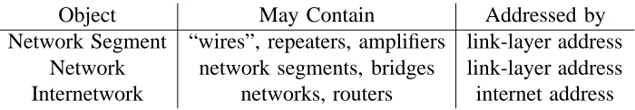
Object May Contain Addressed by
Network Segment “wires”, repeaters, amplifiers link-layer address Network network segments, bridges link-layer address
[image:21.612.150.500.394.455.2]Internetwork networks, routers internet address
Table 1.1: Hierarchy of Network Objects
The various layers described above fall into a hierarchy, from smaller to larger objects,
which is summarized in table 1.1.
These terms are confusing, but most are rooted in history. Attempts to create rational
sets of terminology seem to create even more confusion because they inevitably re-use
old terms for different things. There are equivalent OSI terms for most of these. Most
of them are several words long; they will be avoided in this dissertation.
While we are primarily concerned with analyzing local-area internetworks, it is important
to remember that they are often connected to wide-area networks. The ARPA-Internet is
the largest such packet-switched network in existence today, and has greatly influenced
Arpanet A wide-area network, developed in the 1970’s. It is built out of
point-to-point links and custom-made packet switches called “IMPs” (Interface Message
Processors) which provide connections to hosts and other networks.
ARPA-Internet A very large internet, with thousands of component networks, spanning
most of the United States. It is often referred to simply as “the Internet” (note
capitalization). Until recently, the backbone of the ARPA-Internet was the Arpanet,
which provided most of the long distance communications services. That function
has since been taken over by NSFNet3 and various regional networks such as
BARRNet4.
IP “Internet Protocol”, the underlying datagram protocol used in the ARPA-Internet.
It provides 32-bit internetwork addresses, with variable boundaries between the
network and host part of the address. The network number may be 8, 16, or 24
bits long. The rest of the 32 bits is the host address. IP packets are unreliable;
reliable transport is provided by reliable end-to-end protocols.
IP Network The set of IP addresses with the same network number. IP networks are
defined as class A, B, or C, depending upon whether the network number is 8, 16,
or 24 bits long. This notion of “network” usually bears only a loose correspondence
to the notion of a single link-layer network, as defined earlier. An IP network is a
logical collection of nodes and may be realized with a single link-layer network or
with a complex internetwork. In the later case, each component link-layer network
is termed a subnetwork.
Subnetwork A term used in the ARPA-Internet community that refers to a scheme for
partitioning a single logical IP network into several physical link-layer networks.
With subnet addressing, the host part of an IP address is further subdivided, yielding
a network,subnet,host triple. Subnetting allows an entire internetwork to be
viewed as one IP network. Subnetting is primarily an addressing convenience. By
giving additional structure to an internet address, routers “inside” an IP network
3National Science Foundation Network
can route based upon the subnet number, while routers outside the IP network can
ignore its internal topology.
1.4
Model of Internetworking
With the above terms in mind, the model of networks and internetworks used in this
dissertation is as follows:
An internetwork is composed of networks connected together by routers. Different
networks may use different technologies, e.g. Ethernet, token ring, FDDI, etc.
Each network consists either of one network segment, or several network segments
connected together by bridges. All network segments in a network will usually
be of similar kind. This is because bridges are usually not capable of translating
link-layer addresses for one network type (e.g. Ethernet) into link-layer addresses
for another type (e.g. token ring).
This model is sufficient to describe existing local-area networks, such as Ethernet and
token ring networks. It can be extended to include point-to-point networks by treating
each link as a single network.
1.4.1
Internetwork Maps
“A picture is worth a thousand words,” is an appropriate adage for internetworks. An
internet can be quite complex and can’t be be described concisely with only words.
The best picture of an internetwork is a map showing the component networks, network
segments, routers, and bridges in a compact form. Throughout this dissertation, maps
will be used to illustrate important points.
Figure 1.1 shows a schematic of a simple internetwork composed of a “backbone” network
net1
net6
H Rt
net4
H H Rt
H
net2 net3
H Rt
H
net5
H H
[image:24.612.155.496.120.244.2]Rt
Figure 1.1: Simple Topology Schematic
Note that some networks are Ethernets and some are rings. Most of the area is taken up
by the networks, which clutter the picture.
2 3
4
5
6
Rt Rt
Rt
1
[image:24.612.185.463.333.459.2]Rt
Figure 1.2: Simple Topology Map
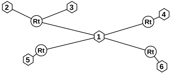
The corresponding map for this topology is shown in figure 1.2. Routers are indicated
by circles and networks are indicated by hexagons. Note especially that the hosts are not
shown on this map. These maps have some interesting topological characteristics that
are discussed in Chapter 3.
Figure 1.3 shows the same network, except that the backbone network is implemented
with three network segments and two bridges (Br). None of the hosts or routers need
know (or, in fact, can detect) that the bridges are there, because they pass the packets
without modifying them.
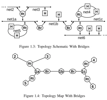
Figure 1.4 shows the corresponding map. Even though this is a complex internet, the
Br
net6
H Rt
net4
H H Rt
H
net1c net1b
net2 net3
H Rt
Br H
net5
H H
Rt
[image:25.612.148.494.112.434.2]net1a
Figure 1.3: Topology Schematic With Bridges
2 3
4
5
6
1a Br
Rt Rt
Rt
Br 1b 1c
Rt
Figure 1.4: Topology Map With Bridges
routers (or bridges) and networks (or network segments), and therefore correspond
di-rectly to network interfaces. This correspondence can be exploited to display additional
information on the map. Figure 1.5, for example, shows relative traffic levels on the
router interfaces by varying the thickness of the corresponding lines. This single map
2 3
4
5
6
1a Br
Rt Rt
Rt
Br 1b 1c
[image:25.612.154.498.121.241.2]Rt
[image:25.612.188.465.541.655.2]shows 40 pieces of information in an easy-to-understand manner. An annotated map like
this will be used to illustrate traffic patterns in Chapter 4.
1.5
Synopsis
My thesis is that the key parameters affecting local-area internetwork “goodness” are
router delay, internetwork topology, and traffic patterns. These are discussed in separate
chapters.
Chapter 2: Router Delay. Although there are many possible causes of
lower-than-desired throughput, most of them can’t easily be changed. One parameter that can
have a significant impact and that is also subject to improvement is router delay.
Router delay is investigated by devising a queuing network model for a router,
evaluating it, and comparing its predictions with delay measurements. The simple
queuing network model does a very poor job of predicting delay. To reconcile
these results, the assumptions and details of the model are investigated in depth.
Chapter 3: Internetwork Topology. The Stanford internetwork started as an ad-hoc
collection of Ethernets, constructed with a little funding by a few academic
depart-ments. When a university-wide networking group was formed to create a more
comprehensive, structured network, the topology was gradually improved to
in-corporate a redundant backbone spanning the entire campus. These changes were
monitored and recorded over a period of two years. Methods for evaluating
redun-dancy and robustness were devised and then tested against the changing topology
of the Stanford internetwork.
Chapter 4: Traffic Patterns. The traffic in the Stanford internet was monitored to
determine which subnetworks communicate the most and which paths are most
heavily used. A few subnets account for most of the traffic in the internet, leaving
Chapter 5: Conclusions. An important meta-issue for all of this research is the design
of networking systems that support monitoring. Besides providing data for analysis,
network monitoring facilities are critical to the operation and maintenance of any
large internetwork. In this chapter, I discuss some of the capabilities which must
be provided by a network monitoring system. I conclude with a summary of the
Router Delay
There are many interrelated factors that determine the speed of data transmission across
an internetwork. As network data rates increase, the delay through routers becomes
the significant limiting factor to network performance, in a local-area context. Intrinsic
network delay, although heavily studied [MB76, AL79, TH80, SH80, Gon85, BMK88],
is a non-issue when routers are added to the system. As we show in this chapter, router
delay is, by far, the largest delay component in the Stanford internet. Furthermore, these
packet delays have a large variance that cannot be attributed to any cause. Such large
variances will adversely affect transport protocols that don’t include variance estimates
in their round-trip time calculations. Router behavior must be carefully examined as
network speeds increase. Our goal is to determine what factors contribute to delay
through a router, and how they can be used to predict actual performance.
2.1
Why are Internetworks Slow?
High delay and limited bandwidth are the two factors that limit a network’s performance
in a particular application. Delay may be more critical in some applications (remote
procedure call) and bandwidth more important in others (bulk data transfer), but these
two parameters suffice to characterize a path between two points in an internet. The two
substantial contributors in a local-area context are intrinsic router delay and delay due to
congestion.
Delay becomes evident when some processing must wait for a response from the other
end before continuing. Most stream protocols do not suffer from this because the “next
data” is known ahead of time and can be sent without waiting for acknowledgment of
the preceding data. Other applications, such as transaction processing or swapping suffer
badly if there is even moderate delay, because some process must wait for one round-trip
for the data to come across the net. These types of applications suffer precisely because
they can’t predict what data they will need ahead of time and must wait one round-trip
to find out. In the absence of better prediction, the only path toward improvement is to
reduce the round-trip time, either by bringing the data closer to the client (fewer hops)
or reducing the delay across each hop (faster routers).
The factors affecting delay and bandwidth are summarized in the following sections.
2.1.1
Speed-of-Light Delay
Electrical signals (in coaxial cable) and optical signals (in optical fibers) propagate at
60-70% of the speed of light, or about 200 meters/uSec. Putting the speed of light into
these units illustrates how significant this delay can be, because one microsecond is a
significant amount of time to a modern computer. A typical local-area internetwork that
spans 2 kM has a speed-of-light delay of about 10 uSec. The delay across the continental
United States (about 3000 miles) is about 24 mSec.1 Even with current technology,
24 mSec is a significant fraction of the total end-to-end delay across the US Internet .
In just a few years, as router performance improves, this immutable delay will be the
dominant delay in wide-area-internetworks.
Speed-of-light delay is almost totally immutable. The only way to change it would be
124 mSec is the theoretical minimum, assuming no repeaters, etc. in the path. Long distance companies
to use a different medium. Except for sending through air or vacuum (microwave or
satellite links), there are no faster mediums available.
2.1.2
Link Bandwidth
Link bandwidth is the rate at which data is sent across a link. Since there may be several
links in a path, possibly with different bandwidths, the smallest bandwidth limits the
bandwidth through the path. Bandwidth affects some network usage more than others. It
adds more delay to larger quantities of data, so interactive terminal or transaction traffic,
requiring small packets of data, won’t notice much difference between a 1 MBit/Sec link
and a 10 MBit/Sec link. File transfer, requiring the movement of hundreds or thousands
of kilobytes of data, will notice the full order-of-magnitude difference.
Link bandwidth is hard to change, once facilities are installed. Even starting from scratch,
there are few choices. Today, in 1990, there are solid standards for what cable to install
for 10 or 100 MBit/Sec, but standards do not exist yet for 1 GBit/Sec networks, even
though such technology is expected to be available in the early 1990s.
2.1.3
Protocol Definition
The definition of a protocol strongly influences its performance in some circumstances.
As a trivial example, a stream protocol that only allows one outstanding packet at a
time will be vastly inferior to a sliding window protocol, at all but the slowest speeds.
Therefore, one sees such simple protocols used for low-speed applications such as file
transfer over slow telephone lines, but rarely over Ethernets. (Deliberately simple boot
load protocols, such as TFTP, are a common exception.)
There are two different potential sources of delay in most protocols today. First, there
is the delay experienced by each packet, every time it passes through a packet switch,
associated with examining and routing that packet. This includes the time taken to do a
address formats, and routing mechanisms all add to this time. Virtual circuit protocols
have less of this overhead and datagram protocols have more.
Second, there is the delay associated with setting up a connection, which may manifest
itself at different levels. In most packet stream protocols, several packets (at least 3) must
be exchanged to establish a connection and get any data across. After the connection
is established, it may take several round-trips to “fill up the pipe” and ramp up to full
bandwidth.[Jac88] As bandwidths increase, per-connection delays represent larger and
larger opportunity costs, when measured in bits. For a 1 GBit/Sec, coast-to-coast network,
the single roundtrip required just to set up connection will be at least as great as the time
required to send 10 MByte of data! Connection set-up and tear-down is more expensive
for virtual circuit protocols than for datagram protocols, although this difference may
change as bandwidths increase and bits (but not round-trips) get cheaper.
These are not insurmountable problems for high-bandwidth, long-distance networks. As
bits become cheap and time becomes precious, trade-offs in protocol design can be made
to get data there early, as well as to quickly estimate the “size of the pipe” so as to be
able to ramp up transmission rate quickly.
Unfortunately, protocol definitions are difficult to change. A large part of the utility of
any network protocol comes with widespread use. So, the most popular protocols, which
might offer the biggest payoff from improvement, are the most difficult to change.
2.1.4
Protocol Implementation
Even the best protocol may not perform up to its potential if the implementation is
poorly done. By design, sequenced packet protocols are able to recover from failures in
the underlying layers, such as lost packets. Because of this resilience, they are often able
to recover from errors in protocol implementations, although performance will almost
certainly suffer. (In fact, this resilience makes it unlikely that subtle errors will be
detected by casual observation.) Some implementations may have actual errors, such as
the next try. More common are subtle tuning errors such as badly set retransmission
timers, that, nevertheless, can wreak havoc in a network.[Jac88]
Protocol implementations can usually be fixed, although it may take some time for fixes
to get distributed. A sufficiently motivated network administrator can make a significant
difference in how quickly such upgrades happen.
2.1.5
Routing Delay
As described above, routers delay packets in several processing steps: packet reception,
header decoding, routing decisions, and packet transmission. If we take the complexity
of these tasks (due to protocol definitions) as a given, there are many different tradeoffs
that may be made when designing a router. High performance may be achieved by
using faster and/or more complex hardware, such as fast CPUs, shared memory for
packet buffers, and multiple processors. Performance may also be improved with clever
software techniques that use routing caches or process packets at interrupt time.
Cut-through is a technique that starts sending a packet before it has been completely received,
once a routing decision has been made, but this requires even more specialized hardware
architectures, in addition to faster components.
Otherwise desirable features, such as security facilities to filter packets based upon source
or destination addresses, add overhead and delay to the processing of each packet. Other
features, such as network management facilities and sophisticated routing protocols add
a background load that can also affect delay.
One important fact to keep in mind is that if a packet must be completely received before
it can be transmitted (as is usually the case, except with cut-through), then a router
will always delay packets by the time it takes to receive a packet, in addition to any
computation that the router must perform. This is a significant delay even for “fast”
networks such as Ethernet; a 1500-byte packet takes 1.2 mSec to receive. This delay is
experienced at each router or bridge in the path and is usually referred to as store and
So, performance (delay) can be traded off against complexity and therefore cost. Routers
are available now over a broad price and performance range, up to 80 or 100 MBit/Sec.
Partridge [Par89] argues that 1 GBit/Sec routers will be achievable very soon.
2.1.6
Network Bottlenecks — Congestion
When more traffic is presented to an internetwork than it can handle, congestion results.
This will produce delay, as packets pile up in routers, where they wait until other traffic
clears. To a single packet stream it will appear that the link’s bandwidth is lower, because
it is now sharing the link with other traffic. The bandwidth reduction is inevitable, but
the delay will be less severe if good congestion control is designed into the network
protocols and routers. [RJ88, Jac88, DKS89]
Although traffic patterns are not instantaneously controllable, a network manager should
keep an eye on what the traffic is doing over the long term. A manager can usually
take some steps to compensate for “hot spots” in the internet, such as rearranging the
topology. If the whole internet is overloaded, that is a different problem — new capacity
must be added, perhaps in the form of higher bandwidth links or better routers.
2.1.7
So What Can We Control?
Many of these parameters are not under the control of the network designer.
Speed-of-light delay and protocol design are certainly not, and the designer has only oblique
influence over protocol implementation. The distance over which the network is to operate
is probably part of the job description. So, the areas of flexibility are: link bandwidth
(technology selection), router delay (product selection) and topology design.
The following tables show breakdowns of end-to-end delay for two scenarios: a
current-technology local-area internetwork and a future-current-technology 1 GBit/Sec wide-area
Local-Area Wide-Area, High-Bandwidth
distance 2 kM 4000 kM
bandwidth 10 MBit/Sec 1 GBit/Sec
avg. packet size 100 bytes 500 bytes
number of routers 2 6
router delay 1 mSec 2 uSec
Table 2.1: Two Sample Internets
The figures for the number of routers in the path are typical of current local-area internet
[Arm88] installations and the NSFnet wide-area internetwork and are on the conservative
side. The local-area packet size is typical of what was seen in the course of this research.
The high-bandwidth packet size is an extrapolation based on trends toward longer
max-imum packet sizes (MTU) in faster networks[Par89], as well as observations of packet
size increases at Stanford. In the past year, the average size has increased from slightly
over 100 bytes to over 200 bytes at many routers. At least some of this increase is due to
the increased network file system traffic across routers. The high-bandwidth router delay
of 2 uSec is based upon estimates of what will be attainable in the near future with fast
processors and specialized architectures, as well as what will be required to be able to
switch 500,000 Pkts/Sec.
The total end-to-end delay, not counting delay in the end-nodes, will be:
TotalDelay Distance Velocity Propagation Delay
Hops RouterDelay Router Delay
Hops 1 PktSize Bandwidth Store & Forward Delay
Local-Area Wide-Area
Propagation Delay 10 uSec 20 mSec
Router Delay 2 mSec 12 uSec
Store & Forward Delay 240 uSec 28 uSec Total Delay 2.25 mSec 20 mSec
Table 2.2: Breakdown of End-to-End Delay
Table 2.2 shows a breakdown of the end-to-end delay for the two sample internets. Each
is the principal component of end-to-end delay. Reducing router delay below 100 uSec
would be less productive, because at that speed transmission delay starts to dominate.
Cut-through then becomes more attractive, although only at significant hardware cost.
In a wide area network, propagation delay swamps all other factors, even if relatively
slow routers are used. In the wide area, there is little point in reducing router delay just
for the sake of reducing end-to-end delay, although delay will certainly be reduced as
routers are made faster to handle the large volume of traffic in higher-speed networks.
2.1.8
End-to-End Delay Variance
The previous section described all of the sources of delay in an internet, and concluded
that, in a local-area context, routers are the major fixed source of delay. Besides the need
for low end-to-end delay, the variance of the delay is also an important factor, especially
for transport protocols.
Transport protocols usually maintain an estimate of the round-trip time and use that
to decide how long to wait before retransmitting a packet. One common choice for
the retransmit timer is just some fixed multiple of the average round-trip time, which
implicitly assumes a fixed delay variance. In this case, a high actual delay variance will
cause some packets to be needlessly retransmitted. The solution to this problem is to
estimate the round-trip time variance as well as the delay.
Another possible consequence of high variance is that some packets may be delayed
enough that newer packets overtake them, resulting in out-of-order packet delivery.
Al-though transport protocols are designed to cope with out-of-order packets, many interpret
an out-of-order packet as a sign that the previous packet was lost, causing more
2.2
Factors Affecting Router Performance
There are three classes of influences on router performance: characteristics of the router,
characteristics of the routed traffic, and external events (besides routed traffic) that demand
the attention of the router. The two routers that I studied are quite different in terms of
these characterizations.
The baseline speed of a router (given the most favorable environment) is determined by
the intrinsic characteristics of the router itself. A router is a complex hardware/software
system. One straightforward characteristic that can be measured is the speed of the
hardware — CPU, backplane or bus, and communication interfaces. The software code
to be executed for each packet is determined by the quality of the implementation and
the complexity of the protocol and routing architecture. The code may also be more or
less constant. If it is constant and small enough to fit into cache memory (if present),
execution speed will be dramatically enhanced. Finally, most routers are complex enough
to require a multi-tasking operating system to handle the variety of tasks the router is
called upon to perform. The selection of the scheduling algorithm, and minimization
of blocking due to critical sections can have a dramatic impact on routing delay. For
example, if a packet to be routed has to wait for an in-process routing-table update to
finish, that packet will likely experience a much longer delay than the average case.
The characteristics of the traffic to be routed also contribute to the delay experienced
by individual packets. Average packet rate and size are important and easy-to-measure
characteristics, but don’t nearly tell the whole story. If packets arrive in bursts, they
will be delayed more than evenly-spaced packets. Burstiness is, unfortunately, hard to
quantify. A useful reference is the Poisson density function, which results in a exponential
distribution of interarrival times. Analytical models often assume Poisson distributions,
providing a baseline for comparison of other results. Unfortunately, real networks do not
exhibit Poisson characteristics [SH80, Llo86, PDA86]. [Llo86] and others have proposed
ways to measure burstiness which, unfortunately, require somewhat subjective parameters
to define what looks “bursty”. In section 2.5.4, I propose a simple technique that allows
2.2.1
Environmental Factors
The environment around a router can also affect the routing delay. Routers are an integral
part of a larger system, and therefore must interact with the rest of the world, besides doing
the primary work of routing packets. Two typical tasks are routing table maintenance
and address resolution. Routing tables are updated by routing update packets, which
are (usually) exchanged between routers. A single router must receive updates and use
them to modify its routing table, as well as send out updates when something significant
changes. A router that communicates directly with many others will spend a lot more
time processing routing updates than a relatively isolated router.
Address resolution is one example of broadcast traffic that routers must handle. In the
Internet, the Address Resolution Protocol (ARP) is used to find Ethernet addresses, given
an IP address on the same network. (ARP is a specific case of address resolution; almost
all internet architectures have some protocol to fill this niche.) A host broadcasts an
ARP request and the host with that IP address responds. The requesting host caches the
response. Some hosts, that aren’t clever enough to do “real” routing, rely on a technique
known as Proxy ARP, where a host blindly sends an ARP request, even if the target host
isn’t on the same network. If a router supports Proxy ARP (most do), then it responds
to the ARP request as if it was the target host (with certain restrictions, mostly that the
router is on a direct path between the two hosts). The originating host then sends packets
destined for the target host to the router, which dutifully forwards the packets. The result,
once the ARP process is done, is exactly the same as if the originating host knew how
to find the appropriate router in the first place.
Proxy ARP works well, except for one thing: participating routers must listen to all ARP
packets on the network and look up each IP address in their routing tables to determine
whether and how to respond. This burden is normally small, unless there are protocol
implementation errors that result in large numbers of ARP requests. Unfortunately, there
are many subtle bugs, in many protocol implementations, that have persisted for years
that produce “storms” of ARP requests[BH88]. Routers are especially vulnerable to such
Finally, other traffic on the networks to which a router connects will interfere with and
delay the transmission of packets. Delay due to contention for the network has been
investigated thoroughly for Ethernets [MB76, AL79, TH80, SH80, Gon85, BMK88].
For situations not involving overloads, this contribution to the total delay is quite small
(typically less than 1 mSec).
2.2.2
Case Studies
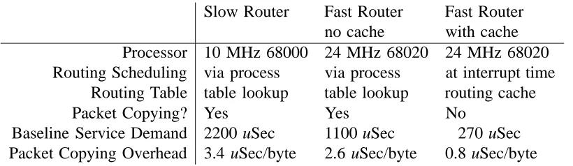
Measurements were made on two different routers, with significantly different
character-istics.
“Slow” Router “Fast” Router Processor 10 MHz 68000 24 MHz 68020 Routing Scheduling via process at interrupt time
Routing Table table lookup routing cache
Packet Copying? Yes No
Typical Delay 2 mSec 100 uSec
Table 2.3: Router Characteristics
Both of these routers use a non-preemptive, priority-based process scheduler. In the slow
router packets are forwarded by a scheduled process (highest priority) which looks up the
destination address in the main routing table. In the fast router, packets are forwarded
by the interrupt handler which looks up addresses in a routing cache. Only cache misses
have to wait for the scheduled process to do a full routing-table lookup. The other major
difference is that packets are copied across the system bus in the slow router, while the
fast router’s two Ethernet interfaces share common packet buffer memory. It is clear from
the delay figures that these techniques pay off well — even discounting the increased
2.3
Queuing Network Model of a Router
The goal of this chapter is to understand the characteristics of a router, specifically, to
model how it delays packets as it routes them. I chose to use a queuing network model
because it is easy to analyze and requires few inputs. I initially use the simplest type
of queuing network model, with one service center, fed by a queue, whose workload
consists of a stream of packets to be routed, as shown in Figure 2.1. After comparing
the predictions of the model to measurements, I identify the significant differences and
attempt to determine their causes.
arrivals departures
queue service center CPU
Figure 2.1: Simple Queuing Network Model
This queuing network model requires one input parameter, the average service demand
at the CPU, which is the amount of time that the CPU must spend to process one packet,
independent of how the time is divided up. That is, it doesn’t matter to the model if a
packet requires two slices of .5 and 1.5 mSec or one slice of 2 mSec. The service demand
is 2 mSec in both cases.
The actual service demand for routing packets was obtained from statistics kept by the
router for the various processes it runs. Figure 2.2 shows an excerpt of the statistics
for the slow router. Statistics are kept on the cumulative runtime and the number of
invocations for each process. The average runtime per invocation is also computed,
although it appears to be severely rounded down in this table. The IP Input process is
the one that does the actual routing in the slow router. (In the fast router, most routing
PID Runtime (ms) Invoked uSecs Process
5 14513508 5754595 2000 IP Input
6 67452 62373 1081 IP Protocols
9 74360 50021 1486 ARP Input
12 2996704 358977 8000 GWINFO Router
14 99964 272581 366 PUP Input
15 64068 271825 235 PUP Protocols
Figure 2.2: Excerpt of Process Statistics
It isn’t sufficient to just look at the average runtime, because when the IP Input process
gets run, there may be several packets in the input queue, which will all be routed on
this invocation. For this reason, the number of invocations will be less than the number
of packets routed. The number of routed packets is obtained from other statistics kept
by the router.
The model inputs we obtained from the router’s statistics were 2200 uSec for a working
router and 2050 uSec for an isolated test router. There is some variation with load, but
not much. We also measured all of the other routers in the Stanford internetwork. Those
running on comparable hardware had estimated service demands between 2000 uSec and
2200 uSec — a reasonably tight range.
2.3.1
Results of the Simple Model
The simple model shown in 2.1 has one parameter, the service demand ( ), and one
independent variable, the offered load ( ) — the arrival rate of packets to be routed.
The closed-form solution to this model[LZGS84, page 109] is quite simple, and produces
three outputs, in terms of the offered load: the saturation packet rate, the average delay
of a packet through the router, and the average number of packets in the system (CPU
and queues):
Saturation rate sat 1
Residence time delay 1
Model Results Asymptote | 0 | 100 | 200 | 300 | 400 | 500 | 600 | 0 | 2000 | 4000 | 6000 | 8000 | 10000
Arrival Rate (Pkts/Sec)
Packet Delay (uSec)
Model Results Asymptote | 0 | 100 | 200 | 300 | 400 | 500 | 600 | 0.0 | 0.5 | 1.0 | 1.5 | 2.0
Arrival Rate (Pkts/Sec)
Number in System
Figure 2.3: Delay and Number in System vs. Offered Load
These results are shown in Figure 2.3 for an example service demand of 2000 uSec. The
two graphs are fundamentally related by Little’s law[LZGS84, page 42], which states that
the average population in the system is equal to the product of the rate at which they
arrive (and depart) and how long each stays in the system: . Little’s law
requires very few assumptions, so it applies to the actual system as well as this simple
model. Therefore, both of these graphs contain exactly the same information. From here
on, we will focus only on the packet delay relationship. If needed, customer populations
can be easily calculated from that.
2.3.2
A More Complete Model
Although the simple model gives intuitively pleasing results for the delay through the
router, it is important to keep in mind the ways that the model and its assumptions deviate
from actual router behavior. Queuing network models, in general, make a number of
assumptions about the characteristics of the system being modeled and its workload. The
Service demand is independent of time. If some aspect of the processor or the
packet load varies with time, such that packets at one time take longer to process
than packets at another time, the model will give poor results. For example, the
model will give bad predictions if the packet size has a strong influence on service
demand and the average packet size varies a lot over time.
Service demand is independent of the load. If several packets arrive close together,
they may be processed by the same invocation of the routing process. All but the
first will be spared the scheduling overhead, reducing the service demand for such
high-load packets.
Packet arrivals have a Poisson distribution. The distribution of packet arrivals
(for a given arrival rate) is a characterization of how much packets bunch up
and determines how much they get in each other’s way, causing queuing delay.
Models that assume a Poisson distribution (such as this one) tend to have simple
solutions. It is well-documented that packet arrivals in packet-switched network
are not Poisson[SH80, Llo86, PDA86]. Our measurements confirm this. The fact
that an actual distribution deviates from Poisson does not, however, say whether
there will be more or less queuing.
In addition, the simple model doesn’t incorporate all of the potentially significant
char-acteristics of the actual router:
The router does non-preemptive scheduling. Although the total amount of time
the processor spends doing other (non-routing) tasks is relatively small,
newly-arrived packets must wait for the current process to finish its task before they
will be processed. Therefore, some non-trivial amount of extra delay may may be
experienced by packets that arrive while the CPU is busy with another task.
Contention delay on output to Ethernet. Packets must wait for the Ethernet to be
idle, and, if the Ethernet is busy, may have to wait for collisions to resolve before
random chance of having to wait for an Ethernet packet to clear can add up to
1.2 mSec to the delay.
Variation in packet characteristics. Any packet characteristic that may make the
router take longer to process the packet. This includes packet size, since it takes
some time to copy the packet when receiving and transmitting. More delay will
be introduced if the packet has to be copied over internal data paths. For Ethernet,
just transmitting the packet can take 1.2 mSec for a maximum-size packet. Packet
destination is another possibility, if routing takes longer for some destinations than
for others.
Routing Ethernet Contention
arrivals departures
Scheduling Delay
(load dependent) (load dependent) (size dependent)
Figure 2.4: More Realistic Queuing Network Model
Figure 2.4 shows a more realistic model that incorporates these differences. In general,
load-dependent and traffic-dependent variations in service demand are difficult to
incor-porate into a queuing network model. If these variations have a significant effect on
delay or queuing, then the model does not have a closed-form solution; it may require
more sophisticated analysis or simulation.
2.4
Router Measurements
We made measurements of delay through a loaded router in regular service in the
Stan-ford network. We used hardware that was identical to the slow router, with two Ethernet
captures all packets on both subnetworks and matches packets departing from one
in-terface of the router with packets that had arrived at the other inin-terface. The data is
recorded and reported to a fileserver via a simple file transfer protocol (TFTP) in real
time. Additionally, the packet trace can be run through a simple simulator, also in real
time, to compare the delay and queueing for each packet in the trace.
Two types of data are returned to the fileserver: packet traces and periodic statistics
reports. For each routed packet, the following information is reported:
Arrival time.
Packet size.
Time since the last routed packet arrived.
Delay through the router, from one network to the other.
Source and destination IP addresses.
Direction through the router.
Information needed to compute the amount of traffic present on the destination
network at the time this packet was transmitted: the number of packets and bytes
since the last routed packet was sent on that network.
In addition, routing update packets and ARP packets (both incoming and outgoing) are
timestamped and reported, to help get a picture of what’s going on inside the router at
particular times.
Besides the packet trace, statistics are reported periodically, typically every one or two
seconds. Most of the statistics are concerned with the volume of traffic (packets/second
and bytes/second) for different types of traffic. From this data, the packet and byte rates,
average size, and average network utilization is computed. Statistics are reported on:
Traffic into and out of the router, for comparison against forwarded traffic.
Traffic forwarded by the router. Average routing delay is also reported here.
Statistics about interface behavior, to help estimate the number of packets not
received because the interface was not ready.
Simulation results, which include statistics about forwarded traffic (as above) as
well as simulated delay and queue length distributions.
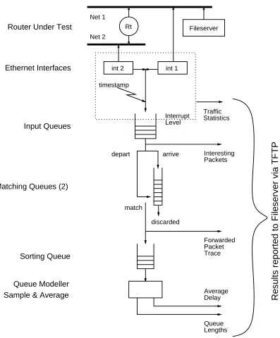
A block diagram of the measuring setup is shown in figure 2.5. The system watches all
packets on both networks and collects the ones that interact with the router. At interrupt
time, received packets are timestamped, essential information is extracted and queued
for processing. The core of the software is the matching queue, which holds records of
packets arriving at the router for later comparison with departing packets. The queue
is limited to a maximum of 50 unmatched packets. At this length, unmatched packets
take between 0.1 and 1 second to be discarded, so this is not a likely source of missed
packets. The general procedure is as follows:
1. ARP broadcasts and routing updates are reported.
2. Forwarded packets are distinguished by the fact that their source or destination
Ethernet address belongs to the router, but the corresponding IP address belongs
to some other host. These packets are classified as either arriving at or departing
from the router and ...
3. Packets arriving at the router are put in a matching queue (one for each direction).
4. Departing packets are matched against packets in the queue. They are matched
based upon source IP address, IP identifier, and IP fragment information. Each
match generates one record of a forwarded packet, with delay computed by
sub-tracting the timestamps.
6. Alternatively, forwarded packets may be processed through a simulator that models
the router queues and computes average delays and queue lengths:
(a) The forwarded packet records are sorted by arrival time (They were generated
based upon departure time.)
(b) The packet records enter a simulator that models queue length inside the
router.
(c) At regular intervals (typically selected as one or two seconds), the average
delay and queue length distribution over the interval is computed and reported
along with other statistics to give a picture of the workload.
This may seem like a lot of trouble to go to just to get this data. The obvious alternative
is to instrument the router code and have the router itself report the data. There are two
fundamental reasons for not instrumenting the router. The most basic reason is that the
added instrumentation would be additional work for the router to do, probably adding
delay and variance. The most compelling reason is that the source code was not available.
Even if it had been, adding the instrumentation would certainly cause some router crashes,
interrupting network service to a very compute-intensive building. The administrators of
the network did not want such disruption; neither did I. The other alternative was to
build an instrumented router and use it to connect a test network, relying on
artificially-generated traffic to provide a workload. However, since the characteristics of “natural”
traffic are one of the unknowns, the realism of the test would suffer.
2.4.1
Measurement Results
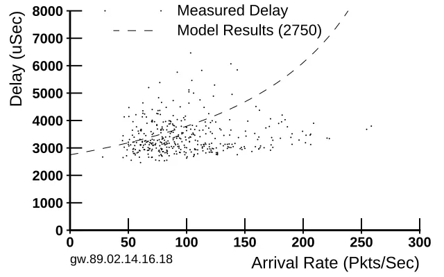
Figure 2.6 shows the results of the measurements, superimposed with the results of the
queuing network model. The queuing network model is evaluated with a service demand
of 2200 uSec, which is indicated in the key. Samples were taken every 2 seconds over
a period of 14 minutes; a typical sample has about one hundred packets. Even with
Net 1
Ethernet Interfaces
Matching Queues (2)
Sorting Queue
Average Delay Queue Lengths
Input Queues Router Under Test
Interesting Packets
Forwarded Packet Trace
Queue Modeller Sample & Average
depart arrive Interrupt Level Net 2
timestamp
Rt Fileserver
int 1
match
Traffic Statistics
discarded
Results reported to Fileserver via TFTP
[image:47.612.130.527.156.636.2]int 2
Measured Delay Model Results (2200)
| 0 | 50 | 100 | 150 | 200 | 250 | 300 | 0 | 1000 | 2000 | 3000 | 4000 | 5000 | 6000 | 7000 | 8000
Arrival Rate (Pkts/Sec)
Delay (uSec)
gw.89.02.14.16.18
Figure 2.6: Delay Measurements — 2 Sec Samples
There is a fairly distinct two-tail pattern, with one tail exhibiting large delay for even
small arrival rates, and the other tail showing relatively low delay, even at high arrival
rates. Both of these tails are at variance with the model, in opposite directions. About
the best thing that can be said about the model’s prediction is that its line passes through
the cloud of points — and then, not even through the middle.
Measured Delay Model Results (2200)
| 0 | 50 | 100 | 150 | 200 | 250 | 300 | 0 | 1000 | 2000 | 3000 | 4000 | 5000 | 6000 | 7000 | 8000
Arrival Rate (Pkts/Sec)
Delay (uSec)
1 Sec
Measured Delay Model Results (2200)
| 0 | 50 | 100 | 150 | 200 | 250 | 300 | 0 | 1000 | 2000 | 3000 | 4000 | 5000 | 6000 | 7000 | 8000
Arrival Rate (Pkts/Sec)
Delay (uSec)
4 Sec
Figure 2.7: Delay Measurements — 1 and 4 Sec Samples