SOIL TEMPERATURE DISTRIBUTION IN BULDANA

JULY-AUG 2016, VOL-4/25 www.srjis.com Page 2567

SOIL TEMPERATURE DISTRIBUTION IN BULDANA

D.A. Kulkarni1 & R.S. Sapkal1

1_{Deptt Chemical Technology Sant Gadgebaba Amaravati University Amaravati (Maharashtra, India)} 2_{Deptt Chemical Technology Sant Gadgebaba Amaravati University Amaravati (Maharashtra, India)}

The objective of this work is to study the monthly and daily variation of soil temperatures at various depths at Buldana. This knowledge will facilitate the suitable placement of Earth-Air Heat Exchanger. A 3-m deep temperature probe was installed in the campus of Rajarshi Shahu Polytechnic, Buldana . Readings were taken over a period of one year. The probe has six temperature sensors, mounted at 60 cm intervals. The probe was buried in a vertical position. The first sensor is at ground level, the second at 0.6 m depth, third at1.2 m, the fourth at1 . 8 cm, the fifth at 2.4 m and the sixth at a depth of 3 m. Temperatures from all the sensors were noted everyday for a year. R eadings were noted in the morning at 8 am, noon at 1 pm and evening at 5 pm. In this paper, the results are presented. Temperatures were noted at intervals of 1 hour on some days in every month.

Introduction

Vidrabha region has widely varying temperatures ranging from 10-12oC in winter to 42-45oC

in summer. People use desert coolers in the summer. These are both water intensive and

power intensive. Both, power and water are scares commodities in this region.

A cheaper alternative and one which does not require the use of water is the Earth Tube Heat

Exchanger. These are in the form of pipes buried deep in the soil. Through the pipes, air is

blown which is cooled by the heat exchanger. The installation of such exchangers requires

the knowledge of soil temperatures at various depths. Temperature data of deep layers of soil

is not available for any site in Vidarbha. Such data for some other places in the country

[1,2.3] have been reported.

To obtain the data in Buldana, a probe which has 6 temperature sensors was installed in the

soil in a vertical position.. The first is at ground level and the others at intervals of 0.6 m with

the last one at 3 m. The temperatures at various depths were recorded daily over a period of 2

JULY-AUG 2016, VOL-4/25 www.srjis.com Page 2568 years. Readings were taken at 5 am, 1 pm and at 6 pm. To obtain the diurnal data, readings

were taken on some days on an hourly basis over a 24 hour period.

The temperature data and a simplified expression for soil temperature distribution is

presented.

The average temperatures (in degrees Centigrade) at various depths over a 12 month period

are as shown in Table 1.

Ground 0.6 m 1.2 m 1.8 m 2.4 m 3.0 m

January 26.27 26 25.2 25.2 25.2 25.2

February 28.46 28.23 27.73 27.6 27.5 27.4

March 32.76 28 27.47 27.3 27 27

April 38.1 29 27.4 27.3 27 27

May 39 29.5 27.43 27.15 27.1 27

June 34.9 28 27.4 27.2 27 27

July 33.3 28 27.5 27.35 27 27

August 29.8 27.5 27.4 27.1 27.1 27

September 30 28.9 27.5 27.1 27 27

October 33.2 27.9 27.5 27.15 27 27

November 30.9 28 27.5 27.15 27.1 27

December 31.5 27.9 27.46 27.1 27 27

Table -1 Average Monthly Temperatures At Various Depths

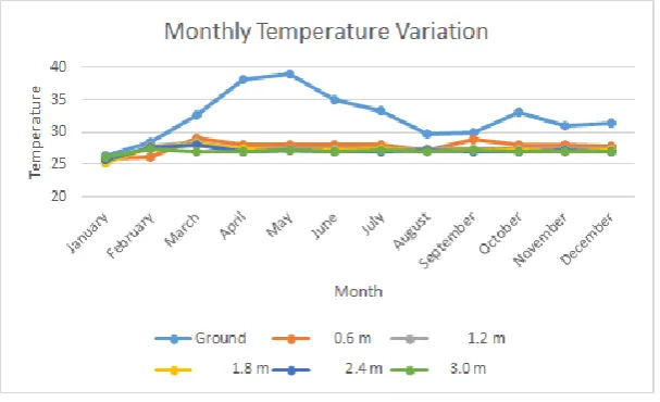
The same data is shown in the form of a graph in Fig. 1

Fig. -1 Average Monthly Temperatures At Various Depths

The annual ground level temperature varied from a minimum of 26.27o_{C to maximum of 39.0}

o_{C. The mean was 32.67} o_{C and the amplitude (difference between the highest and lowest}

JULY-AUG 2016, VOL-4/25 www.srjis.com Page 2569 26oC. The amplitude was reduced to 1.75oC. At 1.2 m depth the temperature varied from 25.2

to 27.73oC with the amplitude being 1.15 oC. At 1.8 m depth there is hardly any change from

the temperatures at 1.2 m depth. At 2.4 m depth the temperature varied from 25.2 to 27.5oC

with the amplitude being 1.15oC. And at the depth of 3.0 m depth the temperature varied

from 25.2 to 27.4 oC with an amplitude of 1.1oC.

The attenuation of the temperature wave is clearly evident, as it penetrates into the soil. It is

also seen that the damping of amplitude with depth is slower as compared to the diurnal

wave.

June to September is the rainy season in Buldana. But the effect of moisture in the soil is felt

only on the surface. At depths of more than 0.6 meters, the temperature varies over a very

narrow range but the phase-lag associated with depth is visible.

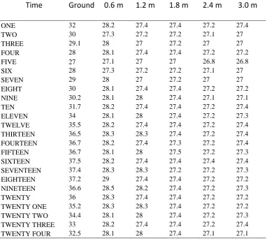
The temperature versus time (ONE means 1 am, TWELVE hours means midday, FIFTEEN

hours is 3 pm and so on) is shown in Table 2.

Time Ground 0.6 m 1.2 m 1.8 m 2.4 m 3.0 m

ONE 32 28.2 27.4 27.4 27.2 27.4

TWO 30 27.3 27.2 27.2 27.1 27

THREE 29.1 28 27 27.2 27 27

FOUR 28 28.1 27.4 27.4 27.2 27.2

FIVE 27 27.1 27 27 26.8 26.8

SIX 28 27.3 27.2 27.2 27.1 27

SEVEN 29 28 27 27.2 27 27

EIGHT 30 28.1 27.4 27.4 27.2 27.2

NINE 30.2 28.1 28 27.4 27.1 27.1

TEN 31.7 28.2 27.4 27.4 27.2 27.4

ELEVEN 34 28.1 28 27.4 27.2 27.3

TWELVE 35.5 28.2 27.4 27.4 27.2 27.4 THIRTEEN 36.5 28.3 28.3 27.4 27.2 27.4 FOURTEEN 36.7 28.2 27.4 27.3 27.2 27.4 FIFTEEN 36.7 28.1 28 27.5 27.2 27.3 SIXTEEN 37.5 28.2 27.4 27.4 27.4 27.4 SEVENTEEN 37.4 28.3 28.3 27.2 27.2 27.3 EIGHTEEN 37.2 29 27.4 27.4 27.2 27.2 NINETEEN 36.6 28.5 28.2 27.4 27.2 27.3 TWENTY 36 28.3 27.4 27.4 27.2 27.2 TWENTY ONE 35.2 28.3 28.3 27.4 27.2 27.2 TWENTY TWO 34.4 28.1 28 27.4 27.2 27.3 TWENTY THREE 33 28.2 27.4 27.4 27.2 27.4 TWENTY FOUR 32.5 28.1 28 27.4 27.1 27.1

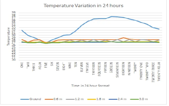
JULY-AUG 2016, VOL-4/25 www.srjis.com Page 2570 Fig. 2shows the above data in the form of a graph It can be seen that the same pattern -

reduction in diurnal fluctuation with depth - was uniformly present through twelve months.

Fig. 2 Temperature variation in 24 hours

Analytical Expression for Daily Mean Soil Temperature :

Consider a semi-infinite medium as shown below. It is assumed that the entire medium is

initially at a constant temperature. Surface of the medium is maintained at a temperature that

varies cyclically.

Let

Z space coordinate (here depth below surface, positive downward) in meters

t time in days

T(z,t) temperature of points at depth z, time t (oC)

Ta temperature of the medium initially (oC), constant

A0 amplitude of the temperature wave at the surface (oC)

ω angular frequency of the temperature wave at the surface (radians/day)

k thermal diffusivity of the material of which the medium is made (m2_/day)

Equation (1) describes one dimensional heat flow through a semi-infinite medium

(1)

JULY-AUG 2016, VOL-4/25 www.srjis.com Page 2571 (2)

Temperature at surface (z = 0) and at time t (t> 0 ) is say

T

Then the variation in temperature at the surface (input) can be expressed as

(3)

where φis the phase lag.

To simplify the expressions, let

Equations 1,2, and 3 can now be written as

(4)

(5)

(6)

where φ is the phase lag

The amplitude of the temperature wave at a depth z is given by the product of amplitude of

the input wave Ao and where the temperature wave number given by

The solution to equation 4 is given in several books on heat transfer [4]

(7)

In terms of original variable T (z, t),

JULY-AUG 2016, VOL-4/25 www.srjis.com Page 2572 The waves are very strongly attenuated. Lower the thermal diffusivity, higher the attenuation.

This is however, a rather simplified view of a complex phenomenon. Soil temperature

depends on many factors which influence the conductive, convective and radioactive heat

exchange between soil and atmosphere. The above equation takes into account only the

unsteady sate conduction through the soil. It is assumed that the soil is homogeneous, which

is generally not the case. Moisture content of the soil varies with depth. This may change the

properties assumed constant here.

To apply equation 8 to the conditions in Buldana, we need to determine Ta , A0, andφ.

Buldana’s climate is considered to be ‘Aw’ according to the Köppen-Geiger climate

classification and the average annual temperature is 30 °C [6]. We will use this as an

approximation of the average soil temperature, Ta.

Amplitude A0 of the annual temperature wave at the soil surface is different for different

seasons. The year may be broadly divided into two parts. February to July is the summer

season and August to January is the winter season. The amplitudes of the annual temperature

wave is different for the two seasons. From the temperature data (Table 1), it is 5.027o for the

summer and 3.26o for the winter. There are two expressions for the two seasons. The value of

φcan be estimated. The peak of the temperature wave at the ground level in a year of 365

days (counted from January) occurs at about day 120 i.e. 1st May. The soil temperature may

be expressed by equation 8 which takes the form

(9)

The parameter α represents the thermo physical properties of soil. The soil in Buldana is

red loamy sand soil with a thermal diffusivity of 0.84-2.36 x 10-6 m2/s [7]

Average thermal diffusivity for red loamy sand soil may be taken as 1.6 x 10-6 m2/s or

0.1382 m2/day. Hence the wave number α works out to 0.2495 m-1. Equation 9 for the

summer and winter seasons can be written as

(10)

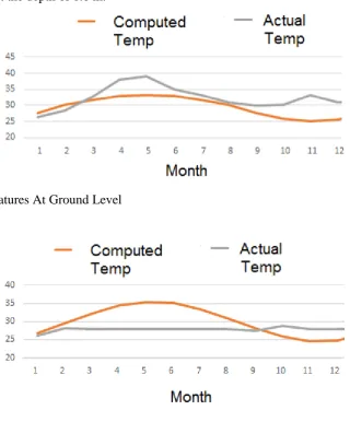
JULY-AUG 2016, VOL-4/25 www.srjis.com Page 2573 The actual temperature and the temperature computed using equations 10 and 11 are shown

in figures 3 and 4. Figure 3 is for the temperatures at the ground level while figure 4 is for

temperatures at the depth of 0.6 m.

Fig. 3 Temperatures At Ground Level

Fig. 4 Temperatures At the Depth Of 0.6 m

Conclusion

1. Measurement of temperature up to the depth of 3-m at Buldanashow that diurnal

fluctuations diminish rapidly with depth and the temperatures at 1.2 m and beyond become

constant. Amplitudes of annual wave too diminish with depth, but less rapidly than the

diurnal.

2. Amplitude of the annual temperature wave at the soil surface is different for the

summer and the winter seasons. The temperature computed using the equations 10 and 11

JULY-AUG 2016, VOL-4/25 www.srjis.com Page 2574 The strata between 1.2 m to 1.8 m is suitable for installation of earth-air tube heat exchanger.

The soil temperatures do not decrease appreciably at greater depths. Also the cost of making

a trench for the pipes increases with depth without any material change in amplitude.

References

‘Soil temperature regime in arid zone of India’ Krishnan A. and GGSN Rao Arch. Met. Geoph. Ser. B, 27, 15-22, 1979

‘Thermal Regime Of Mollisols Under High WaterTable Conditions’. Tripathi R.P. and B.P. Ghildyal Agricultural Meteorology, 20, 493, 1979

Soil Temperatures Regime at Ahmedabad G. Sharan and R. Jadhav www.iimahd.ernet.in/publications/data/2002-11-02GirjaSharan.pdf

‘Fundamentals of Heat and Mass Transfer’ T. L. Bergman, A.S. Lavine, F.P. Incropera and

D. P.DeWitt 7th Ed., March 2011,John Wiley & Sons, Inc

http://en.climate-data.org/location/767151/

‘Ground Water Information Buldhana District’ M.K. Rafiuddin Report by Central Ground Water Board, Maharashtra, page 9, 2013

‘Comparison Of Thermal Properties Of Three Texturally Different Soils Under Two Compaction Levels’P. Pramanik and P. Aggarwal