IMAGE DUPLICATION AND ROTATION DETECTION METHODS FOR STORAGE UTILIZATION

(1)

ISSN:1992-8645 www.jatit.org E-ISSN:1817-3195

CHARACTERISTICS OF DUAL-CORE PHOTONIC CRYSTAL

FIBER BY FD-BPM

1

HICHAM CHIKH-BLED,2BOUMEDIENE LASRI,1MOHAMMED EL-KEBIR CHIKH-BLED

1_{University Abou-Bekr Belkaid , Faculty of Technology, Laboratory of Telecommunications (LTT),}

Tlemcen, Algeria 2

University Dr Moulay Tahar, Faculty of Sciences, Laboratory of theoretical physics of Tlemcen (LPT), Saida, Algeria

E-mail: [email protected] ,[email protected] ,[email protected]

ABSTRACT

We present results related to the numerical method based on Finite Domain Beam Propagation Method (FD-BPM). It allows to characterize microstructured fibers Air / Silica (FMAS) with a good approximation. We also show how optogeometrical parameters (d: diameter of the holes,Λ: spacing between the air holes) can influence the propagation characteristics for applications in optical networks Telecommunications.

Keywords: Finite domain beam propagation method (FD-BPM), Modeling, Microstructured fibers Air/Silica (FMAS), Diagrams of dispersion, Couplers, mode coupling.

1. INTRODUCTION

Microstructured fibers Air/Silica (FMAS), also referred to Photonic Crystal Fibers (PCF), consisting of a central defect region (typically solid silica) surrounded by multiple air holes running parallel to the fiber length have been one of the most significant achievements in optical technology within the last years.

The microstructured fibers arrived today at maturity, and allow to consider improving the performance of fiber components for optical telecommunications. The FMAS with two cores have applications in several applications such as filters, multiplexers and couplers [1].

The beam propagation method has been applied to many wave guiding structures in guides wave optics [2-3] and tool that allowed us to model the FMAS, the standard form of implementation of the FD-BPM is the Crank-Nicholson method.

2. FORMULATION

Many numerical tools exist to model the behavior of a FMAS [4-5].

Our choice has been on the FD-BPM (Finite Domain Beam Propagation Method) based on the Crank-Nicholson algorithm. This method has the advantage of being less intensive computing ressources.

The problem of light propagation in waveguides with arbitrary geometry is very complicated in

general, and it is necessary to make some approximations.

We will assume an harmonic dependence of the electric and magnetic fields [6], in the form of monochromatic waves with an angular frequency , in such a way that the temporal dependence will be of the form . The equation which describes such EM waves is the vectorial Helmholtz equation:

∇ + ( , , ) = 0

Where = ( , , ) denotes each of the six Cartesian components of the electric and magnetic fields.

The refractive index in the domain of interest is given by ( , , ), and will be determined by the waveguide geometry (optical fiber, directional coupler,...etc)

If the wave propagation is primarily along the positive direction, and the refractive index changes slowly along this direction, the field

( , , ) can be presented as a complex field

amplitude ( , , ) of slow variation, multiplied by a fast oscillating wave moving in the + direction:

( , , ) = ( , , )

Where = / is a constant which represents the characteristic propagation wave vector, and as the refractive index of the substrate.

(1)

(2)

Journal of Theoretical and Applied Information Technology 10thSeptember 2015. Vol.79. No.1

Substituting the optical field in the Helmholtz equation [6], it follows that:

− + 2 = + + ( − )

Where = 2 / denotes the wavevector in the

vacuum and ( , , ) = ( , , ) has been

introduced to represent the spatial dependence of the wavevector.

If we also assume that the optical variation is slow in the propagation direction SVEA (Slowly Varying Eenvelope Approximation) we will have:

²

² ≪ 2

We can ignore the first term on the left-hand side of equation (3) with respect to the second one, this approximation is known as parabolic or Fresnel approximation and equation (3) leads to:

2 = ²

²+ ²

² + ( − )

Which is known as the Fresnel or paraxial equation. It is the starting equation for the

description of optical propagation in

inhomogeneous media, and in particular, in wave-guide structures. An example is TE propagation in 1D waveguides, where the Fresnel equation reduces to:

2 = ²

² + [ ( , ) − ]

Where is the only non-vanishing component of the electric field associated to TE modes of the 1D waveguide, and where the refractive index is represented by n(x, z). The solution to the Helmholtz equation or the Fresnel equation applied to optical propagation in waveguides is known as the beam propagation method (BPM) [6]. Two numerical schemes have been proposed to solve the Fresnel equation. In one of them, optical propagation is modelled as a plane wave spectrum in the spatial frequency domain, and the effect of the medium inhomogeneity is interpreted as a correction of the phase in the spatial domain at each propagation step [7]. The use of the fast Fourier techniques connects the spatial and spectral domains, and this method is therefore called fast

Fourier transform BPM (FFT-BPM). The

propagation of EM waves in inhomogeneous media can also be described directly in the spatial domain by a finite difference scheme (FD) [8]. This technique allows the simulation of strong guiding structures, and also of structures that vary in the propagation direction. The beam propagation method which solves the paraxial form of the scalar wave equation in an inhomogeneous medium using the finite difference method is called FD-BPM.

The Helmholtz scalar wave equation in partial derivatives is approximated by a finite difference scheme [6], which can be expressed as:

2 ( + ∆ ) − ( )_∆

= ( ) − 2 ( ) + ( )

∆ ² + ( − ) ( )

Where ( ) is the optical filed at the position ( ∆ , ). This scheme in finite differences, known as “forward-difference”, allows us to calculate the optical field ( + ∆ )after a propagation step∆ from a knowledge of the complete field ( )at the position [9].

The calculation of ( + ∆ ) from equation (7) is simple, and indicates that the optical field ( + ∆ ) can be computed from field values

( ), ( )and ( )at a given position z.

Besides, from a numerical point of view it is a conditionally stable method, where the stability condition is given by:

∆ ≪∆

2 = ∆ ²

An alternative way to overcome this problem consists in using a finite difference scheme somewhat similar to the former known as “backward-difference” [9]. The Helmholtz scalar takes the following form:

2 ( + ∆ ) − ( )_∆

= ( ) − 2 ( + Δ ) +_{∆ ²} ( + Δ )

+ ( − ) ( + Δ )

(3)

(4)

(5)

(6)

(7)

(8)

(3)

(17)

(15)

This method has the advantage of

unconditionally stable, while the approximated solution obtained in the simulation is similar to the “forward-difference” method, consequently no more accuracy is gained.

There is a method, also based on finite difference schemes, that is not only unconditionally stable but also provides more accurate solutions than the two previous methods, this method called Crank-Nicholson scheme [9-6], is a linear combination of the “forward difference” method and the “backward-difference” method.

The finite difference method following a Crank-Nicholson scheme for solving the paraxial propagation equation can be represented as:

[2 + Δ ] ( + Δ )

= [2 − Δ (1 − ) ] ( )

The operator is defined as:

≡ − 2 +_∆ + ( − )

Expanding this scheme in terms of finite differences, the following equation is obtained:

2 ( + ∆ ) − ( )

= ( − ) ( + ∆ ) − (1 − ) ( ) ∆

+ ( + ∆ ) − 2 ( + ∆ ) +_∆ ( + ∆ )

− (1 − ) ( ) − 2 ( ) +_∆ ( ) ∆

This equation relates the optical field at( + ∆ ) that is( + ∆ ), with the field at , that is, ( ).

Readjusting terms in the previous equation, one obtains:

( + ∆ ) + ( + ∆ ) + ( + ∆ )

= ( )

Where the coefficients , , and are defined by:

= − ∆

∆ ²

= 2 _{∆ ²}∆ − ∆ ( + ∆ ) − +

2

= − _{∆ ²}∆

= (1 − )_∆∆ ( ) + ( )

+ (1 − )∆ ( ) −

− 2(1 − )_{∆ + 2}∆ ( )

It can be demonstrated that the solution to this equation system shows an excellent numerical stability, the algorithm used for solving this tridiagonal system is the Thomas Method [9], which requires a computational time that increases with N, while the time required for obtaining a fast Fourier transform using a grid of N points increased as N log2 N.

The Crank-Nicholson scheme is unconditionally stable for α > 0.5 if the refractive index is independent of x and z. Nevertheless, if the refractive index varies slowly or if it is uniform with small discontinuities, the Crank-Nicholson method can be applied locally. Under these circumstances, the analysis leads to valid solutions even for the most adverse situations.

Apart from the numerical stability, the greatest advantage of the Crank-Nihcolson method comes from the fact that it provides a better approximation to the exact solution of the problem.

The finite difference method is a powerful numerical method which allows the use of large propagation steps, with the consequent saving in computational time.

3. DIAGRAMS OF DISPERSION

The FMAS is characterized by the following parameters :Λ = 2.5 , = 1.6 .

To simulate the propagation of the field, we chose the following space step of discretization: ∆ = ∆ = 0.25 in the transverse plane and Δ = 0.5 along the axis of propagation.

The index profile in Figure 1 is calculated for the plane z=0.

(10)

(11)

(12)

(13)

(4)

(17)

3.1 Effective Index Versus the Wavelength

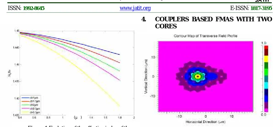
The Figure 2 shows the changes in the effective index of the fundamental mode in the FMAS calculated with the BPM method versus wavelength for different values of /Λ.

The diameter of the holes varies from the = 1 to 3.5 and the spacing between the air holes is fixed which is equal toΛ=4 .

In the last figure show that the effective index decreases in a linear way when the ratio d/Λ increases, for short wavelengths the intensity of the mode is highly concentrated in the material constituting the which is the silica, the effective index tends towards the value of the refraction index of silica. For large wavelengths the intensity of the mode spreads in the microstructured cladding and the effective index tends towards

(Fundamental Space filling Mode).

Note that the effective index varies greatly from 1.434 to 1.444 depending of the wavelength, for short wavelengths the light is confined in the core increasing the effective index of the cladding. For example d/Λ=0.4, the light penetrates more strongly into the holes which will cause a drop in the effective index of the microstructured cladding.

The Figure 3 shows the changes in the effective index of the fundamental mode in the FMAS versus the wavelength for different pitchesΛ(Λ = 2.5µm to Λ = 4.5µm) and with diameter of the holes d=1.5 µm.

The decrease is stronger for lower values of Λ, this characteristic of the FMAS rises from the strong variation of the index of the microstructured cladding.

We also note that the longer period Λ is large between the holes the effective index tends to converge to the index of silica is 1.45. For short wavelengths the light is confined in the core of the FMAS.

The Figure 4 shows the changes in the effective index of the fundamental mode in the FMAS versus the wavelength for different diameter of the holesd (d = 1µm to d = 3.5µm) and with spacing between the air holesΛ = 4µm.

(µ )

nef

[image:4.612.60.315.72.265.2]

f

Figure 2: Evolution of the effective index of the fundamental mode versus wave length for different

[image:4.612.309.524.337.491.2]

values ofd/Λ

Figure 3: Evolution of the effective index of the fundamental mode versus wavelength for different

values of

nef

[image:4.612.60.289.405.575.2]

f

Figure 1: Index profile of FMAS type RTIM

(µ )

nef

f

(5)

Figure 5:Evolution of the effective index of the fundamental mode versus the ratios d/Λ for

different pitches

We note the effective index decreases with the growth of the wavelength and for small diameter of the holes approximately 1 the effective index tends to converge to the index of silica.

It is at the origin of the great diversity of the characteristics of propagation of the FMAS. 3.2 Effective Index Versus the Ratios d/

From Figure 5 we note that the effective index varies considerably from 1.375 to 1.443. It’s noted that the effective index decreases linearly when the ratio d/Λincreases.

A variation of the effective index of the high way is the choice of pitch between the air holes. When the value ofΛincreases we notice that the effective index will be close the index of silica is 1.45.

4. COUPLERS BASED FMAS WITH TWO

CORES

Introducing two adjacent defects (2 cores) in the cladding of the FMAS, as shown in Figure 6 the energy transfer between two cores [10]. This component can be used as a power splitter or an optical switch. The FMAS is characterized by the following parameters:

Coupling energy results from the superposition of the evanescent fields from each core.

4.1 Influence of the Diameter d of the Holes and the Period of the Coupling Length

The abacque of dispersion in Figure7 shows the change of the coupling length versus diameter of the holes to different values ofΛ. The parameters of the FMAS with 2 cores are: diameter of the

[image:5.612.78.524.68.276.2]

(µ )

Figure 4:Evolution of the effective index of the fundamental mode versus wavelength for different

values of

/Λ

nef

f

Figure 6: Energy transfer between 2 cores

[image:5.612.315.548.459.635.2]

Diameter of holes d (µm)

(6)

(18)

(19) core dc=0.6µm, nsilica=1.45, the wavelength used is

=1.55µm. We note that low coupling lengths can be obtained by reducing the period Λ, or the diameter d of the holes.

4.2 Influence of Diameter dcon the Coupling Length

The parameters of FMAS are Λ=2.4 µm, nsilica=1.45 and d variable. Note that the diameter of the central hole affects the coupling length. For a minimum coupling length we must be choose a diameter of core dclow as can be seen in Figure 8.

5. FIELD DISTRITION IN A FMAS WITH TWO CORES

The Figure 9 and Figure 10 below represent the profiles of the electric field, the electric field carthographies and profile of the electric field (3D) in the fundamental mode respectively for FMAS 2 cores.

The distance for which the amplitude of the second core is maximum is defined as the coupling length Lc, theoretically this distance is obtained from the propagation constants of the even and odd modes resulting from the coupling between the evanescent field from each core.

The analytical expression [11] for this parameter is given by:

= ₋ _{= 2(} ₋ ₎

Where and are the propagation

constants of the even and odd modes of propagated mode.

The coupling coefficient is deducted from the coupling length Lc:

/ = 2

/

0 50 100 150

0 0.1 0.2 0.3 0.4 0.5 0.6 0.7 0.8 0.9

20

40

60

80

100

120

140

20 40 60 80 100 120 140 20

40

60

80

100

120

140

20 40 60 80 100 120 140

C

o

u

p

li

n

g

l

en

g

th

Lc

(µ

m

)

[image:6.612.315.531.174.424.2]

Diameter of core dc(µm)

Figure 8 : Coupling length versus the diameter of the core for different air holes d

Λ=3µm, d=0.8µm Λ=3µm, d=1µm

Λ=3µm, d=1.2µm Λ=3µm, d=1.6µm

Figure 9: Profile Of The Electric Field For Different Diameters Of The Holes

Λ=3µm, d=0.8µm Λ=3µm, d=1µm

[image:6.612.66.293.271.425.2]

Λ=3µm, d=1.2µm Λ=3µm, d=1.6µm

[image:6.612.320.521.502.704.2]

(7)

ISSN:1992-8645 www.jatit.org E-ISSN:1817-3195 It is observed from these results that smaller the

diameter increases the better confinement of the power in the two cores of the FMAS. We also note the diameter d=0.8 µm (about /2), an appearance of a secondary maximum of both sides of the maximum is probably due to a diffraction phenomenon.

Finally, for a hole diameter of the order of 1.6 µm (approximately ), the quantity of air in the cladding is larger, and there is less optical power transported by the latter.

6. CONCLUSION

The simulation tool FD-BPM has enabled us to model and estimate the properties of FMAS based optogeometrical parameters. These new generation fibers are the basis of new optical functions. However BPM simulation method has limitations due to the rectangular meshing and introduces it in the choice of the steps of discretization.

A study of the coupling between modes of a dual-core FMAS was discussed to highlight the power exchange. This property has allowed us to present a new component that is power diveder coupler based

FMAS with 2 cores.

We could identify the parameters which allow to obtain the most significant propagation properties. Abacques dispersion of the effective index were calculated and presented.

REFERENCES:

[1] K. Saitoh, Y. Sato, and M. Koshiba, “Coupling characteristics of dual-core photonic crystal fiber couplers,” Opt.Express, 11, pp. 3188-3195, 2003.

[2] M.D. Feit and J.A. Fleck, Jr. “Computation of mode properties in optical fiber waveguides by a propagating beam method,” Appl. Opt., vol. 19, no. 7, pp. 1154-1163, 1980.

[3] D. Yevick and B. Hermansson, “New formulations of the matrix beam propagation method: Application to rib waveguides,”IEEE J. Quantum Electron., vol. 25, no. 2, pp. 221-229, 1989.

[4] W. Huang, C. Xu, S. T. Chu, and S. K. Chaudhuri, “A Vector beam propagation method for guided

wave optics,’’ IEEE J. of Photon. Tech., 3, pp. 910-913, 1991.

[5] F.Brechet, J.Marcou, D.Pagnoux, and P.Roy “Complete analysis of the characteristics of propagation into photonic crystal fibers, by the finit

element method” Opt. Fiber Technol, vol. 6, pp. 181-191, 2000.

[6] G.Lefante, “Integrated Photonics” ISBN 0-470-84868-5

[7] M.D. Feit and J.A. Fleck, “Light Propagation in Graded-Index Optical Fibers”, Applied Optics, 17, 3990–3998 (1978).

[8] R. Scarmozzino and R.M. Osgood,

“Comparison of Finite-Difference and Fourier- Transform Solutions of the Parabolic Wave Equation with Emphasis on Integrated Optics Applications”, Journal of the Optical Society of America A, 8, 724–731 (1991).

[9] W.H. Press, S.A. Teukolsky, W.T.

Vetterling and B.P. Flannery, Numerical Recipes in Fortran 77: The Art of Scientific Computing, Chapter 12, Cambridge University Press, New York (1996).

[10] Daru Chen; Gufeng Hu; Lingxia Chen, “Dual-core Photonic Crystal Fiber For Hydrostatic Pressure Sensing,” Photonics Technology Letters, IEEE, vol.23, no.24, pp.1851, Dec.15,2011