Robust estimation of multivariate location and scatter with application to financial portfolio selection

University of London

Robust Estimation of Multivariate

Location and Scatter with Application to

Financial Portfolio Selection

Simona Costanzo

London School of Economics and Political Science

PhD thesis

UMI Number: U615245

All rights reserved

INFORMATION TO ALL USERS

The quality of this reproduction is dependent upon the quality of the copy submitted.

In the unlikely event that the author did not send a complete manuscript and there are missing pages, these will be noted. Also, if material had to be removed,

a note will indicate the deletion.

Dissertation Publishing

UMI U615245

Published by ProQuest LLC 2014. Copyright in the Dissertation held by the Author. Microform Edition © ProQuest LLC.

All rights reserved. This work is protected against unauthorized copying under Title 17, United States Code.

ProQuest LLC

789 East Eisenhower Parkway P.O. Box 1346

A b stract

The thesis studies robust m ethods for estim ating location and scatter of multi­

variate distributions and contributes to the development of some aspects regarding

the detection of multiple outliers.

A variety of m ethods have been designed for detecting single point outliers which,

when applied to groups of contam inated data, lead to problems of “masking” , th a t

is when an outlier appears as a “good” data. R obust high-breakdown estimators

overcome the masking effect, also allowing for a high tolerance of “bad” data. The

Minimum Volume Ellipsoid (MVE) and the Minimum Covariance D eterm inant es­

tim ator (MCD) are the most widely used high-breakdown estim ators.

The central problem when identifying an anomaly is setting a decision rule. The

exact distribution of the MCD and MVE is not known, im plying th a t the diag­

nostics constructed as a function of these robust estim ates have also an unknown

distribution. Single point oultiers can be recognized using M ahalanobis distances;

m ultivariate outliers are detected by robust (via MCD and MVE) distances of Ma­

halanobis type. The thesis obtains the small sample distribution of the first ones in

an alternative simpler way th a n the proof existing in the literature. Furthermore,

some empirical evidences show the need of a correction factor to improve the ap­

proximation to the expected distribution. Some graphical devices are suggested to

enhance the results.

One of the limiting aspects of the literature on robustness is the lack of real d ata

applications beside the literature examples. The personal interest in financial sub­

jects has driven the thesis to consider applications in this area. P articular attention

is paid to m ethods for optim al selection of financial portfolios. M ean-Variance port­

folio theory selects th e assets which maximize the return and minimize the risk of

the investment using M aximum Likelihood Estim ates (MLE). However, MLE are

known to be sensitive to relatively small fractions of outliers. Furtherm ore, a wide

To m y frien d Paolo

“II mare imm enso, Toceano mare, che infinito corre oltre ogni sguardo, Tim m ane mare onnipotente -

c }e un luogo dove finisce, e un istan te - Vimmenso mare,

un luogo piccolissim o e un istan te da nulla. ”

Acknowledgements

During these years of research, when the motivation for completing the PhD has not always been ’’strong”, I have found support and inspiration from many people.

I thank Sankarshan and George who made my start at the LSE smooth and enjoyable.

My thanks go to the whole LSE Statistics Department, with special mention to Dr Martin Knott and Dr Irini Moustaki, who have been an irreplaceable sup­ port. “Obrigada” to my friend and office mate Teresa, with whom I shared many difficulties encountered during research.

The project was sponsored by BSI (Banca della Svizzera Italiana) to whom I am immensely indebted. My thanks go particularly to Alberto Di Stefano, Andrea Laurent, Fabiano Cavadini, Fransiska Bignasca. Dr Fabio Trojani, from University of Lugano, Switzerland, gave an important contribution to the original idea for the project.

I am grateful to my family who has pushed me to follow my aspirations without any limitations.

I thank my encouraging friends from Italy: Anna, Bettina, Claudia, Giada. Thanks to Yasmine for taking care of social life in London when I was still a

“fresher”: the thesis was written despite her distractions.

C ontents

1 Introduction 1

1.1 The Outlier P ro b le m ... 2

1.2 Contribution of the T h e s is ... 3

1.3 The O u tlin e ... 6

2 A Financial D ata Set 9 2.1 Introduction... 9

2.2 Data D e scrip tio n ... 10

2.3 Com m ents... 11

3 Background for Robust M ultivariate E stim ation and Computa­ tional Issues 18 3.1 Basic C o n c e p ts ... 18

3.2 Aland 5-Estimators ...23

3.3 The MVE and MCD Estimators: the General Id e a ...25

3.4 The MVE and MCD Estimators: Some P ro p erties... 27

3.5 MCD Estimator: Computation ... 29

3.5.1 Forward Search for the Choice of the Initial S e t ...32

3.6 Conclusions ...34

4 D etection o f M ultivariate Outliers 37 4.1 Introduction...37

4.2 Standardized R esiduals...38

4.2.1 Deletion R e s id u a ls ... 39

4.3.1 Out-of-sample M D ... 41

4.3.2 Deletion MD ... 43

4.3.3 In-sample M D ... 44

4.4 Robust M D ... 48

4.5 Simulation Envelopes for Robust and Mahalanobis D istances... 49

4.6 Further Empirical E v id e n c e ... 51

4.7 A Monte Carlo T e st... 52

4.7.1 The Test R e s u lts ... 54

4.7.2 Accuracy of the R e s u l t s . . 55

4.8 Robust Envelopes for Outlier D etection...56

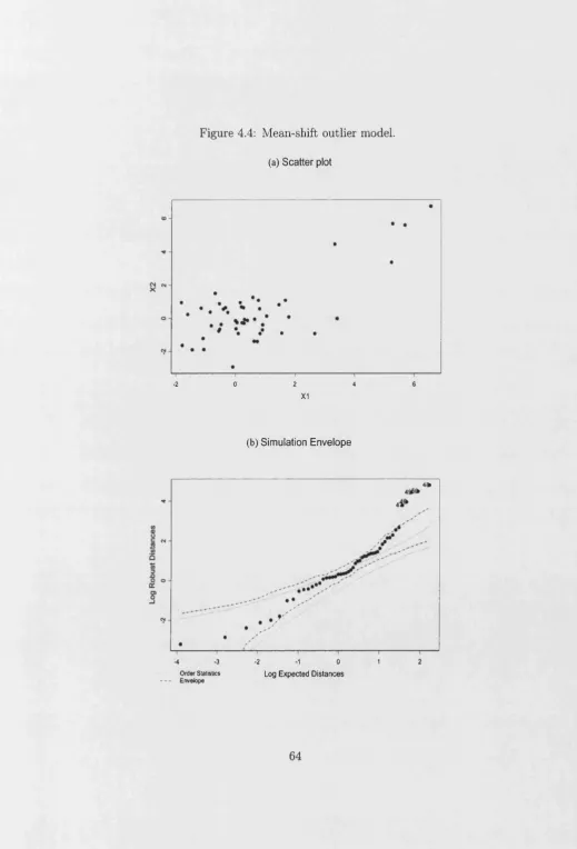
4.8.1 The Mean Shift Outlier M odel...56

4.8.2 Example 1: Modified Wood Gravity Data . ... 57

4.8.3 Example 2: Hawkins, Bradu and Kass D a t a ... 58

4.8.4 Example 3: Stack Loss D a t a ...59

4.9 C onclusions... 59

5 R o b u st D etectio n o f O utliers using th e S tu d e n t-t d istrib u tio n 70 5.1 Introduction... 70

5.2 The Multivariate Student-t Distribution ... 71

5.3 Maximum Likelihood E s tim a tio n ... 72

5.3.1 Distribution of p>MLE and 4? m l e... 74

5.4 The EM algorithm: general id e a ...75

5.4.1 ML estimation with known degrees of freed o m ...77

5.4.2 ML estimation with unknown degrees of f r e e d o m ... 78

5.5 Empirical Results on p>MLE and SFm l e... 79

5.6 Outlier Diagnostics: Weighted Mahalanobis D istances...81

5.7 Example 1: Univariate Linear Regression on Stackloss D a t a 82 5.7.1 Example 2: Stackloss D a ta ... 84

5.7.2 Example 3: Hawkins, Bradu and Kass ...84

6 R obust M odelling for Financial Portfolio Selection 95

6.1 Introduction... 95

6.1.1 Basic Notions on Financial P o rtfo lio s... 95

6.1.2 N otation... 97

6.2 Standard Mean-Variance Portfolio Problem ... 98

6.2.1 Motivations for a Robust M o d e l...101

6.2.2 The Robust M odels... 102

6.3 The Influence of Outliers on Markowitz Portfolio...103

6.4 The W eights... 106

6.5 Performances: Turnover, Risk and R e t u r n ...108

6.5.1 Performances for the Normal and Outlier-shift m odels 108 6.5.2 Performances for the Multivariate-t M o d e l...109

6.6 Out-of-Sample performances... 110

6.7 Conclusion... I l l 7 Conclusions 126 7.1 The Results of the Thesis ... 126

7.2 Suggestions for further S tudies... 128

List o f Tables

1.1 Huber’s data (a) and residuals from the linear (lm), quadratic (qm) and linear without outlier fits (b)-(d)... 8

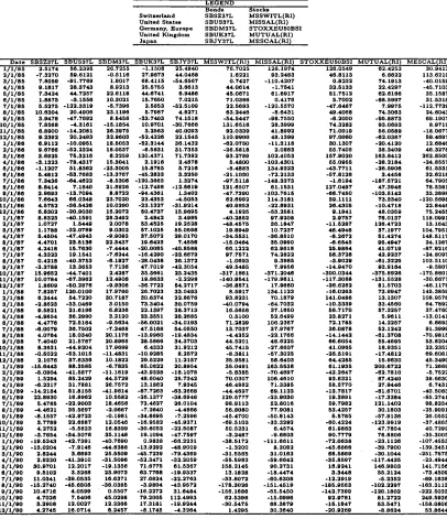
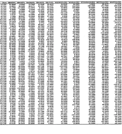
2.1 Monthly stock and bond indexes (yt). Source: Data Stream, BSI. . . 12 2.2 Monthly stock and bond indexes (yt). Source: Data Stream, BSI. . . 13 2.3 Monthly stock and bond indexes (yt). Source: Data Stream, BSI. . . 14 2.4 Annualized return data su m m ary ... 14 2.5 Annualized return data correlations... 14

4.1 Average and median proportion of observations lying outside the tol­ erance ellipse of xj,0.975... 52

4.2 Proportion of rejections for the AD test on Mahalanobis Distances (MD) and Robust Distances (RD). The unweighted RD are obtained from the MCD estimates not reweighted for efficiency. The size of the test is a for 1000 replications. S is the proportion of observations fitted robustly. ...60

5.1 Minimum and maximum (.) bias for fa mle and *&mle on a multi­ variate Student-t with v = 3. t3 is estimated by fixing the degrees of freedom... 87 5.2 Minimum and maximum (.) standard deviation for P>mle and ^ m le• 87

5.3 Bias of the first two elements of the estimated location vector of a simulated multivariate Student- 1... 88 5.4 Bias of the first diagonal and off-diagonal elements of the estimated

5.5 Efficiency of the first two elements of the estimated location vector of a simulated multivariate Student- 1 ... 88 5.6 Efficiency of the first diagonal and off-diagonal elements of the esti­

mated scatter matrix of a simulated multivariate Student- 1... 88 5.7 Minimum and Maximum bias and efficiency of the MLE for fi and VP

on a simulated multivariate Student-t with v = 3... 89 5.8 Bias and efficiency of the MLE for the first two elements of fi and

a diagonal and off-diagonal element of ^ obtained from a simulated multivariate Student-t with v = 3...89 5.9 Estimates from fitting a regression on Stackloss D ata... 90 5.10 Results from the fit of the multivariate Student-t model on Stackloss

Data... 90 5.11 Results from the fit of the multivariate Student-t model on Hawkins,

Bradu and Kass data...90 5.12 Example 1: Stackloss data. Weights of the t3 model. The odd

columns are the observations; the even columns the weight values. . . 92

6.1 Turnover, return and risk of the tangency and global minimum vari­ ance portfolios from a simulated Normal distribution without outliers. Risk free rate= . 2 ... 113 6.2 Turnover, return and risk of the tangency and global minimum vari­

ance portfolios from a simulated Normal distribution with 10% out­ liers. Risk free rate= .03 (m o n th ly )...113 6.3 Turnover, return and risk of the tangency and global minimum vari­

ance portfolios from a simulated multivariate Student-t distribution with 3 degrees of freedom. Risk free rate= .003 ... 114 6.4 Out-of-sample performances on four assets portfolios. Risk free rate=

. 0 3 ... 114

6.5 Sensitivity of the robust MCD model performances to h, the size of the fitted set. The proportion of the “good” observations in the simulated data is 0.9. Risk free rate= .03 (monthly), p= 4...115

6.6 Sensitivity of the robust M-t model performances to the fitted degrees of freedom. Risk free rate= .03 (monthly), p= 4... 115 6.7 Out-of-sample performances of the tangency portfolio on a real data

List o f Figures

1.1 Huber’s data example: scatter-plot, (a), and Q-Q plots, (b)-(d). . . . 8

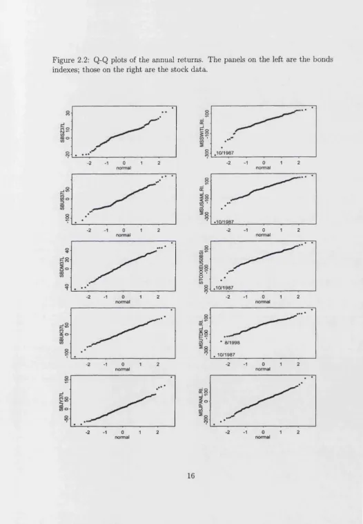
2.1 Autocorrelation function for annual return data. Squared total return for Swiss bonds (a), squared total return for Swiss stocks (b), absolute total returns for Japanese bonds (c) and cube total returns for UK bonds (d)...15 2.2 Q-Q plots of the annual returns. The panels on the left are the bonds

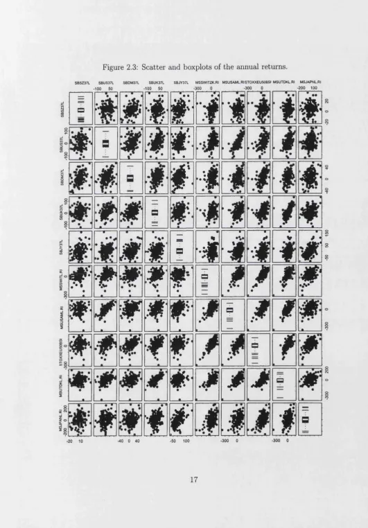
indexes; those on the right are the stock data...16 2.3 Scatter and boxplots of the annual returns... 17

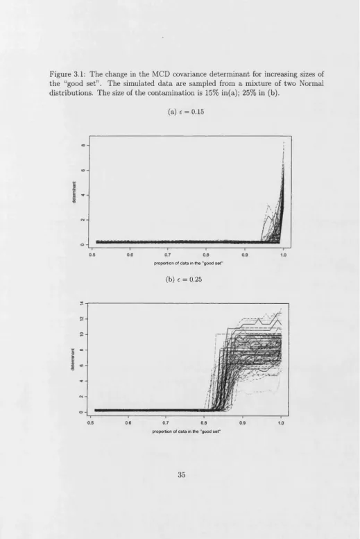
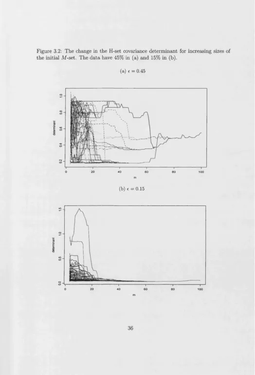
3.1 The change in the MCD covariance determinant for increasing sizes of the “good set”. The simulated data are sampled from a mixture of two Normal distributions. The size of the contamination is 15% in(a); 25% in (b)... 35 3.2 The change in the H-set covariance determinant for increasing sizes

of the initial M-set. The data have 45% in (a) and 15% in (b)... 36

4.1 Q-Q and Box Plots for Mahalanobis and robust distances in three independent samples from a simulated Normal distribution... 61 4.2 97.5% Simulation envelopes for Mahalanobis and robust distances

generated from simulated Normal data and theoretical order statistics

of the Xp... 6 2

4.3 Quantile plots for mean and median of robust and Mahalanobis dis­ tances... 63 4.4 Mean-shift outlier model ... 64

4.5 Example 1, Woodgravity data... 65 4.6 Example 1, Woodgravity data, simulation envelopes... 66 4.7 Example 2, Hawkins, Bradu and Kass data... 67 4.8 Example 2, Hawkins, Bradu and Kass data, simulation envelopes. . . 68 4.9 Example 3, Stackloss data...69

5.1 Determinant for the sample variance-covariance matrix of a simulated multivariate Student-t data. The dimensions of the sample varies from 20 to 200 observations on 4 variables... 91 5.2 Maximum, 99, 98.5, 98 and 97.5% simulation envelopes for Maha­

lanobis distances on multivariate Student-t data... 91 5.3 Plot of the sorted weights (f) from the t3 model... 92 5.4 Profile Likelihood for the multivariate Student-t degrees of freedom. . 93 5.5 Plot of the sorted weights for the multivariate Student-i with v = 3

fitted on Stackloss Data... 93 5.6 D-D Plot of Mahalanobis-type Distances fitted on Bradu Hawkins

and Kass data. The solid lines is the 97.5% Chisquare quantile. . . . 94

6.1 Portfolio frontiers... 116 6.2 Contaminated and outlier-free portfolio mean-variance frontiers. . . .117 6.3 Influence function for the ML mean of the global minimum-variance

portfolio from a bivariate Normal distribution and a Student-t 118 6.4 Influence function for the ML variance of the global minimum-variance

portfolio from a bivariate Normal distribution and Student-t... 119 6.5 Distribution of the weights for Merton’s model (6.3)-(6.5) on Normal

data. n=200, p=4, q=12% annual... 120 6.6 (a) Average mean-variance fro n tiers...121 6.7 (a) Average mean-variance fro n tiers...122 6.8 Bias for the average fi and for the determinant of \fr for increasing

6.9 Average standard deviation for the MLE on a multivariate Student-t. The sample size varies from 80 to 800 observations, the number of

replications are 120... 124

C hapter 1

Introduction

The word robustness is widely used in many fields of scientific research to signify the most diverse meanings. Scientific experiment are constructed according to a framework which determines the validity of the results. Sometimes these initial assumptions are too restrictive and do not match what happens in reality. In general, the results of an experiment are termed robust if they are not affected by changes in the initial framework. This section clarifies the meaning of statistical robustness and how it is related to outlier diagnostics.

Huber (1981) defines the word robust as

insensitive to small deviations from statistical assumptions.

Hampel, Ronchetti, Rousseeuw, and Stahel (1986) restrict the concept of robustness in the following way:

robust statistics, as a collection of related theories, is the statistics of approximate parametric methods.

between semiparametric and robust models, we believe that, in general terms, the former models allow for a wider range of distributions than the latter models. Fur­ thermore, while semiparametric methods model all the data, the robust statistics reject the observations believed to be inconsistent with the reference model or, at least, reduce their importance through down-weighting. There are various impli­ cations on the properties of the robust and semiparametric estimators which can be studied referring to the specific literature: Bickel, Klaassen, Ritov, and Wellner (1993), Horowitz (1998), Powell (1994). For the reasons explained above, Hampel’s definition seems more appropriate than the Huber’s to describe the robust tools studied in this thesis.

The approximations of parametric models are determined by gross errors that are measurement or transcription errors, distributional mis-specifications, rounding or grouping, or by the presence of some correlation structure in the data. These errors generate outliers or “strange” observations. The outlier diagnostic literature is vast and includes many different approaches mainly depending on the model considered. Most of the studies concern regression models, although there is an increasing amount of work on time series and categorical data.

1.1 T h e O utlier Problem

The most common definition of an outlier is

an observation lying far from the rest of the data,

although this is not sufficient to identify an anomaly. A remote observation is an outlier only if it is judged inconsistent with the remainder of the data. The purpose of statistical methods is to introduce some objectivity in the identification and treatment of the “strange” points.

Regarding the treatment of outliers, rejection of strange points is not always the optimal solution. The most common criticism from the “antagonists” of robust methods is that blind deletion could result in a loss of some relevant information. Simply, if these points are generated from errors in reading, recording or grouping,

they should be eliminated from the data. In other cases, when the anomalies derive from a different probability distribution or a different deterministic model, there are various approaches for treating the outliers other than plain deletion. A first approach consists in applying a transformation, when possible and appropriate, in order to adapt the model to the furthest points. A second approach is to reduce the importance of outliers through down-weighting.

Huber’s data offers a simple and clear example of how even only one distant observation can influence the model’s fit. The observations are only six for each of the two variables (Table 1.1). A linear model, y = X T/3, where y is the ( 6 x 1 ) response vector and X the (6 x 2) matrix of carriers, including the dependent variable and a constant term, is fitted. Panel (a) suggests that there might be one outlier, observation 6, in the direction of the x axis. These types of outliers are called leverage points. It is also an influential observation since it changes the direction of the fitted fine. Panels (b) and (c) are the Q-Q Normal plots of the residuals from a linear and quadratic fit: yi = J2l=o Pkxii * = 1,2, ...,6. The second fit appears to be a better solution than the first one: the residuals lie closer to the straight line. A good result comes also from fitting a straight fine after the deletion of the “bad” observation shown in panel (d). Further investigations are needed to decide between the two approaches. In addition, the data axe not enough to show if the

extreme point is an outlier or simply a sample vaxiation of the data.

The meanings of some terms that will be recurrent in the thesis have been implic­ itly defined. An extreme observation is a point fax from the rest of the data. This is an outlier if the distance is considered “unusual” . There axe different types of anomalies according to how these points are related to the model considered: lever­ age points and influential observations (sometimes called good and bad leverage points) are outliers for a regression model.

1.2

C ontribution o f th e T hesis

regarding the detection of multiple outliers. The computational work is substantial. Large use is also made of graphical tools, which are the most direct and simple approach to detect anomalies.

The identification of multivariate outliers is a particularly difficult topic to cope with. A variety of methods have been designed for detecting single point outliers which, when applied to groups of contaminated data, lead to problems of “masking” (meaning when an outlier appears as a “good” datum). Robust high-breakdown esti­ mators overcome the masking effect, also allowing for a high tolerance of “bad” data. On the contrary, most of the robust statistics have breakdown at a fraction l / ( p + l ) of contaminated data, where p is the dimension. Therefore, high-breakdown estima­ tors are particularly useful in high dimensional sets. Many different methods have been offered by the literature as well as feasible algorithms for their computation. The Minimum Volume Ellipsoid (MVE) and the Minimum Covariance Determinant estimator (MCD) are the most popular ones (Chapter 3). The second one has better statistical properties than the first one, but its use has been limited by the lack of a fast and efficient algorithm. There are three main algorithms developed for the computation of MCD estimates: the FSA (Feasible Solution Algorithm) by Hawkins (1994) is computationally heavy and relatively slow; the Fast Algorithm (Rousseeuw and Van Driessen 1999) solves problems of speed; and the Forward Search for the MCD (Atkinson and Cheng 2000) applies a simple and efficient criterion. In addition to increasing the velocity of the algorithm on which various authors seem mostly focused, there are other computational aspects to be discussed. The first one is the choice of the size of the starting subset which is the outlier-free set. Including too few data in the initial set can compromise the efficiency of the estimates. However, if we start with too many data, including outliers, the result is a loss of robustness. We discuss this problem and propose some practical solutions.

Robust methods allow us both to find estimates for the location and the variability of a multivariate cloud according to robustness criteria and to detect groups of outliers at the same time. The central problem when identifying an anomaly is setting a decision rule. In this context, the distributional aspects of the robust diagnostics become very important. The asymptotic properties have been studied

in the literature, although the exact distribution of the MCD and MVE is not known. This implies that the outlier diagnostics constructed as a function of the robust estimates also have an unknown distribution. Single outlying points can be recognised using Mahalanobis distances as a diagnostic tool; multivariate outliers are detected by the robust (via MCD and MVE) distances of Mahalanobis type (Chapter 4). The thesis obtains the small sample distribution of the Mahalanobis distances in an alternative simpler way than the proof existing in the literature. Furthermore, some empirical experiments show the need of a correction factor for the approximation of the robust distances to their asymptotic distribution. Simulation envelopes, introduced for the first time by Atkinson (1985) in regression models, are found to be a valuable tool to detect outliers, overcoming the problems deriving from the unsatisfactory approximation of the robust distances by the theoretical distribution.

It has been noted that one of the limiting aspects of the literature on robust­ ness is the lack of real data applications beside the canonical examples th at are usually referred to by experts in the topic. My personal interest in financial sub­ jects has driven the thesis to consider applications in this area. In particular, the

the high transaction costs. All these points motivate the construction of a robust portfolio selection model as proposed in the thesis.

It has been mentioned that stock returns follow a non-gaussian distributional model. Although various authors disagree on the specific distribution, the common idea is that returns are longer-tailed than the Normal. The Student-t is suggested as a possible model. The advantages of using such a distribution compared to other long-tailed forms derive mainly from its simplicity and closeness to the Normal. The thesis explores the possibility of robust modelling using the multivariate Student-^ and compares it with the high-breakdown optimizer. Some distributional aspects of the estimates are also discussed.

1.3

T he O utline

Chapter 2 explores a financial data set which will be often used in the thesis. The literature regarding robust estimators of multivariate location and scatter is reviewed in Chapter 3, with particular attention to the MVE and the MCD estimators. This Chapter also examines some computational aspects of the MCD method regarding the choice of the size of the initial set.

The detection of groups of outliers in multivariate data is studied in Chapter 4. The diagnostics used in the literature are reviewed and the distribution of Ma­ halanobis distances is analytically derived. The critical regions commonly used to detect outliers in a multivariate data set are quantiles of the Chisquare. It is shown that this approximation leads to the rejection of too many points, with a consequent loss in efficiency of the estimator. Analytical and empirical evidence are provided.

Chapter 5 studies an alternative way of modelling robustly via the Student- t distribution. Obtaining the MLE for a multivariate-^ requires the use of the EM algorithm traditionally used when there are some missing observations in the data assumed Normal and non-contaminated. The EM can also be adapted to the framework of the multivariate t distribution. Finally, detection of multiple outliers is explored and the goodness of this model is compared in some applications with the high-breakdown estimator methods.

The robust construction of a model for optimisation of portfolios is proposed in Chapter 6. The Chapter provides analytical and empirical motivations for the use of a robust model. The performances of the model are analysed through a simulation study and an example using real data.

re

s

id

u

a

ls

Table 1.1: H uber’s d ata (a) and residuals from the linear (lm), quadratic (qm) and linear w ithout outlier fits (b)-(d).

observation x y residual (lm) residual (qm)

1 -4 2.48 2.09 0.25

2 -3 0.73 0.41 -0.26

3 -2 -0.04 -0.27 0.05

4 -1 -1.44 -1.59 -0.44

5 0 -1.32 -1.39 0.42

6 10 0.00 0.75 -0.01

Figure 1.1: H uber’s d ata example: scatter-plot, (a), and Q-Q plots, (b)-(d).

(a) (b)

in e a r fit w ith o u t o b s 6

8 10 o

•1.0 -0.5 0.0 0.5 1.0

Q u a n tile s o f S ta n d a rd N orm al

(C) (d)

•1.0 -0.5 0.0 0.5 1.0

o

2 13

■g 9o

9

•1.0 -0.5 0.0 0.5 1.0

C hapter 2

A Financial D a ta Set

2.1

Introduction

This Chapter introduces a data set coming from a real investment decision problem. The data is a recurrent example in the thesis. It consists of 10 monthly price indexes of the bond and stock markets. For each type of asset, there are indexes on 5 coun­ tries: United Kingdom, Japan, USA, Germany and Switzerland. The bond market indexes are provided by Salomon and the stock data by Morgan Stanley, with the exception of the stocks for Europe, produced by BSI (Banca della Svizzera Italiana). The observations are 175: from January 1985 to July 1999 and are expressed in local currencies.

The interest is on returns rather than asset prices. Therefore, each variable has been transformed applying differences of logarithms of the prices in two subsequent times:

yt = ln(pt_i/pt),

2.2

D ata D escription

There is a considerable amount of financial literature describing financial return data, particularly stocks. These are shown to be longer tailed than the Normal distribution and weakly autocorrelated.

Our data are indexes and, therefore, better behaved than series of single stocks. There are no significant autocorrelations of order one, although it is still possible to find some correlations of higher order or of some function of the initial variables (Figure 2.1). This means that the observations are not independent, although, as a first approximation, they will be treated as such.

Since we assume the assets are time independent, the scatter-matrix plot is a very useful graph to display the data structure and the relationship between pairs of variables. On the diagonal panels, there are the box-plots for each asset-market. The bond distribution is symmetrical and approximates quite well the Normal. The stock indexes are roughly symmetrical, but more scattered than the Normal distribution. These results are confirmed by looking at the Q-Q plots of Figure 2.2 and at Table 2.4. The skewness and kurtosis in Table 2.4 are computed using moment sample estimates:

* - ! W

'

* - [iK^T]-3’

where y is the average return and o is the sample standard deviation. Values around 0 indicate that the distribution is symmetric and mesokurtic. The kurtosis coefficient is positive for all the stocks, which means that the distribution is leptokurtic. The negative 71 shows that the distribution of the stocks is also skewed to the left, which

is confirmed by the Q-Q plots.

The panels in the off-diagonals are scatter-plots of each pair of assets. These show high correlation among the stock markets (the last five rows and column panels). The bonds appear less highly associated, although the pairwise correlation

coefficients are still significant (Table 2.5). The only exception is the Swiss bond index, which appears to be significantly related to the German bond one.

Both the scatter and the Q-Q plots evidence a couple of observations lying far from the bulk of the data. This confirms what we expected: because the data are monthly indexes (weighted averages of single stocks resulting from aggregations of daily data) there are only a few outliers. October 1987 represents the well known crash of the New York Stock Exchange, the largest drop of the returns after 1929, which affected most of European and Asian markets. August 1998 represents the Russian crisis, following the crash of the Asian markets, which extended to Europe and the US.

2.3

C om m ents

Table 2.1: Monthly stock and bond indexes (yt ). Source: Data Stream, BSI. L E G E N D

B o n d s S to c k s S w itz e r la n d S B S Z 3 7 L M S S W I T L (R I ) U n ite d S t a t e s S B U S 3 7 L M I S S A L ( R I ) G er m a n y , E u r o p e S B D M 3 7 L S T O X X E U 5 0 B S I U n ite d K in g d o m S B U K 3 7 L M U T U A L ( R I ) J a p a n S B J Y 3 7 L M E S C A L (R I )

D a t e S B S Z 3 7 L S B U S 3 7 L S B D M 3 7 L S B U K 3 7 L S B J Y 3 7 L M S S W I T L (R I ) M I S S A L ( R l) S T O X X E U 5 0 B S I M U T U A L ( R I ) M E S C A L (R I ) 1 / 1 / 8 5 2 .5 1 7 4 5 6 .2 3 9 5 2 6 .7 2 5 5 -1 .1 5 0 8 2 5 .4 8 4 0 7 6 .7 0 2 5 1 2 6 .1 9 7 4 1 2 6 .0 5 4 9 6 2 .4 2 5 3 3 0 .9 4 1 3 2 / 1 / 8 5 - 7 .3 2 7 0 5 9 .6 1 2 1 -0 .5 1 1 6 2 7 .9 8 7 3 4 4 .0 4 6 8 1 .6 2 2 1 9 3 .2 4 8 3 4 6 .8 1 1 3 6 .8 6 2 2 1 1 3 .6 2 1 9 3 / 1 / 8 5 7 .8 0 5 9 - 9 1 .7 7 6 9 1 .9 0 1 7 6 8 .4 1 1 5 • 5 4 .6 5 6 7 0 .7 4 2 7 - 1 1 0 .4 2 0 7 0 .8 2 3 2 7 4 .1 9 1 3 -4 0 .0 1 5 9 4 / 1 / 8 5 9 .1 8 1 7 2 8 .3 7 4 3 8 .9 2 1 3 2 5 .5 7 5 5 3 .0 6 1 3 4 4 .0 6 1 4 -1 .7 5 4 1 3 2 .5 1 3 3 2 2 .4 2 9 7 • 4 5 .7 1 0 3 5 / 1 / 8 5 7 .3 4 2 4 4 4 .7 2 5 7 2 2 .6 1 1 8 4 4 .6 7 4 1 6 .9 4 8 6 4 5 .0 6 7 1 6 1 .6 9 1 7 5 1 .7 5 1 2 6 2 .6 1 6 6 3 5 .1 5 8 7 8 / 1 / 8 5 1 .6 8 7 5 - 3 .1 5 5 6 1 0 .3 0 2 1 1 5 .7 6 5 0 7 .0 2 1 5 7 1 .0 3 8 6 0 .4 1 7 6 5 .7 0 0 2 - 6 8 .5 9 9 7 3 1 .5 3 1 8 7 / 1 / 8 5 5 .5 2 7 5 -1 2 2 .3 3 1 9 -5 .7 3 9 6 2 .5 8 5 3 -5 2 .5 1 0 9 2 2 .5 6 9 3 - 1 2 0 .5 5 7 0 -4 7 .6 4 6 7 7 .9 9 7 5 - 1 1 2 .7 7 3 9 8 / 1 / 8 5 1 0 .6 3 0 4 2 0 .4 9 0 6 2 3 .1 1 9 6 5 .7 6 8 7 4 .8 2 7 1 6 3 .2 4 4 6 -8 .6 4 3 1 4 9 .4 0 6 8 7 4 .3 0 6 3 2 4 .6 0 4 3 B / l / 8 5 3 .9 4 7 8 - 4 7 .7 6 9 2 8 .5 4 5 6 -3 3 .7 4 0 3 7 4 .1 5 1 8 - 5 4 .5 4 4 7 -9 8 .7 5 5 0 - 6 .2 0 0 0 -9 5 .8 8 7 3 6 9 .1 9 0 7 1 0 / 1 / 8 5 7 .8 5 6 8 -4 .3 1 6 1 - 1 5 .1 8 5 4 1 0 .9 7 0 1 - 3 0 .7 6 6 6 1 3 1 .6 5 1 6 2 8 .3 9 9 9 7 4 .3 2 8 2 9 3 .0 6 9 3 8 .9 7 1 9 1 1 / 1 / 8 5 6 .8 6 0 0 - 1 4 .2 0 8 1 2 6 .3 9 7 5 3 .2 5 6 3 4 0 .0 0 9 3 9 2 .0 3 3 9 4 1 .8 9 9 2 7 1 .0 0 1 9 5 6 .0 5 8 9 -1 8 .0 6 7 7 1 2 / 1 / 8 5 9 .2 3 9 2 2 0 .2 4 9 3 3 2 .9 6 0 3 -5 2 .4 2 2 6 2 2 .1 5 4 5 1 1 0 .9 9 0 0 4 8 .1 3 9 9 9 7 .0 0 6 0 -0 2 .0 3 8 7 5 9 .4 6 9 7 1 / 1 / 8 8 6 .9 1 1 2 -1 0 .0 9 5 1 1 8 .5 0 5 3 • 5 2 .3 1 4 4 3 6 .1 4 3 2 - 6 2 .0 7 5 0 -1 1 .3 1 1 8 3 0 .1 3 0 7 - 2 0 .4 1 2 0 1 2 .6 8 4 6 2 / 1 / 8 8 9 .6 7 6 6 - 5 2 .2 3 2 4 1 8 .0 5 3 7 -6 .5 8 3 1 3 1 .7 3 5 3 - 2 6 .5 8 1 8 2 .0 8 8 3 5 5 .7 4 0 5 3 8 .3 4 0 9 4 6 .3 2 7 8 3 / 1 / 8 8 3 .6 9 2 5 7 6 .3 2 1 6 6 .2 2 5 9 1 3 0 .4 3 7 1 7 1 .7 3 8 2 9 3 .2 7 6 9 1 0 2 .4 0 5 3 1 5 7 .9 0 2 0 1 6 3 .8 4 1 2 2 6 2 .8 5 0 0 4 / 1 / 8 8 - 3 .1 3 2 3 - 7 8 .4 3 1 7 1 5 .3 0 4 1 2 .1 9 1 6 2 .4 8 7 8 5 .4 8 0 0 -1 0 3 .4 3 0 1 6 5 .0 9 5 5 - 2 8 .2 1 8 4 -2 4 .8 5 5 7 5 / 1 / 8 8 - 1 .1 2 0 7 5 1 .8 3 6 2 - 2 3 .3 0 0 5 1 5 .8 7 8 5 5 .7 2 1 6 - 8 .4 8 8 3 1 3 4 .9 3 2 3 - 4 3 .7 7 1 1 - 2 6 .5 9 0 0 6 1 .5 3 3 1 8 / 1 / 8 8 5 .4 8 1 2 - 5 3 .7 6 8 3 • 1 3 .3 7 6 7 - 4 5 .2 8 2 3 3 .3 2 5 0 • 2 1 .1 0 3 0 -7 2 .2 1 3 3 - 5 7 .8 1 2 8 3 .4 4 5 8 3 2 .6 2 1 8 7 / 1 / 8 8 7 .3 4 3 6 -6 4 .4 6 2 2 -8 .5 3 0 6 -1 2 0 .3 6 6 5 1 .3 2 7 4 -9 7 .5 1 1 8 -1 4 8 .3 3 7 3 - 1 .0 1 9 4 - 1 8 7 .5 7 2 1 6 4 .7 9 0 5 8 / 1 / 8 8 8 .8 4 1 4 7 .1 8 4 0 2 1 .6 9 2 6 - 1 2 .7 4 9 8 -1 2 .6 6 1 9 1 2 1 .6 5 0 7 6 1 .1 5 3 1 1 2 7 .0 4 9 7 4 7 .3 9 4 6 7 8 .5 3 8 1 0 / 1 / 8 8 2 .9 6 9 3 - 1 3 .7 0 9 4 8 .8 7 2 2 -9 4 .4 3 6 1 1 .3 4 0 2 -4 7 .7 3 9 0 - 1 0 3 .7 6 1 5 -6 6 .7 4 5 0 -1 0 3 .5 1 4 2 3 3 .3 8 9 8 1 0 / 1 / 8 8 7 .6 6 4 3 6 6 .0 3 4 8 2 3 .7 0 2 0 2 3 .4 3 5 3 -4 .5 0 5 3 6 2 .6 9 9 2 1 1 4 .3 1 8 1 3 9 .1 1 1 1 7 3 .3 3 4 0 - 1 2 0 .5 6 9 8 1 1 / 1 / 8 8 4 .5 7 5 2 -3 6 .6 4 2 6 1 0 .0 2 9 0 - 2 3 .1 3 2 7 - 3 1 .9 2 1 4 4 0 .9 8 5 3 - 2 2 .8 9 3 1 2 6 .4 3 0 5 -1 0 .4 7 1 8 2 2 .8 4 4 6 1 2 / 1 / 8 8 6 .8 3 0 2 -2 0 .9 0 3 0 1 5 .2 0 7 2 5 0 .4 7 3 7 1 5 .9 6 9 5 4 .1 9 2 5 - 5 3 .2 5 8 1 9 .1 0 4 1 4 8 .0 3 6 9 7 5 .2 4 5 5 1 / 1 / 8 7 8 .8 3 2 3 -4 0 .1 5 9 1 2 8 .3 4 9 2 2 .4 8 4 2 3 .4 9 8 5 - 4 0 .2 8 5 2 9 7 .9 2 0 8 2 .9 7 5 7 7 6 .0 1 3 7 1 1 8 .0 9 9 1 2 / 1 / 8 7 1 .0 7 2 7 1 .5 4 4 9 2 .0 0 7 8 5 3 .4 5 2 5 1 9 .2 5 2 8 -4 8 .4 5 7 5 3 6 .1 8 4 7 -1 1 .5 2 8 7 1 2 0 .4 7 2 3 1 3 .1 6 4 3 3 / 1 / 8 7 1 .1 7 8 8 -3 2 .0 7 8 9 9 .0 3 0 2 5 7 .1 0 2 6 5 6 .0 5 9 8 1 9 .8 9 4 9 1 0 .7 2 3 7 4 6 .4 9 4 6 3 7 .1 9 7 7 1 0 4 .7 9 5 1 4 / 1 / 8 7 6 .4 5 0 4 - 4 7 .4 9 4 3 -9 .9 0 9 3 3 7 .6 0 7 2 2 9 .0 1 7 0 -3 4 .5 5 3 1 - 3 6 .8 5 1 0 - 8 .2 6 7 2 6 1 .4 2 7 4 1 4 8 .5 1 1 7 8 / 1 / 8 7 4 .4 7 0 1 2 3 .5 1 3 6 2 2 .3 4 3 7 1 9 .6 4 2 3 7 .4 5 5 6 -1 5 .0 4 6 4 3 6 .0 9 9 0 - 6 .6 5 4 5 9 5 .4 9 4 7 2 4 .1 2 6 7 C / l / 8 7 4 .2 4 1 8 1 5 .7 6 3 0 -7 .4 4 4 4 • 2 0 .0 0 8 5 - 4 0 .8 5 8 8 6 6 .1 2 2 2 6 2 .9 6 1 8 2 5 .9 8 8 4 4 1 .0 7 1 9 - 8 7 .9 2 1 6 7 / 1 / 8 7 4 .3 3 2 3 1 9 .1 5 4 1 -7 .6 2 4 4 - 1 6 .4 2 9 0 -2 3 .6 6 7 9 9 7 .7 5 7 1 7 4 .2 8 2 2 5 8 .3 7 2 8 4 2 .9 2 3 7 -2 4 .8 0 9 7 8 / 1 / 8 7 0 .4 2 1 8 -4 0 .3 7 5 3 - 6 .1 9 2 7 • 2 8 .0 4 3 8 2 6 .1 3 7 2 - 1 .0 6 9 3 9 .3 9 8 5 -3 .9 0 2 9 -6 1 .3 2 2 9 1 0 3 .5 1 1 0 8 / 1 / 8 7 - 3 .3 7 8 8 1 3 .3 6 5 3 7 .7 1 3 0 4 7 .7 0 1 9 -4 2 .3 0 5 4 4 9 .5 4 8 5 7 .9 9 5 6 • 1 4 .9 4 7 0 9 3 .9 1 6 4 - 9 .5 8 0 7 1 0 / 1 / 8 7 1 5 .9 6 5 2 -4 4 .7 4 0 1 2 .4 2 8 7 3 5 .5 6 6 1 2 3 .2 4 3 5 - 3 1 7 .1 8 6 1 -3 7 1 .2 0 4 6 -3 0 0 .0 3 4 4 - 3 7 5 .8 9 2 6 • 1 7 5 .8 8 0 1 1 1 / 1 / 8 7 1 0 .0 7 8 4 -6 7 .3 9 6 2 1 2 .4 9 0 6 1 9 .8 6 3 3 -2 .2 2 9 8 - 1 4 0 .9 5 4 1 -1 7 9 .9 6 1 1 - 1 1 7 .3 0 8 8 - 1 3 1 .5 5 2 8 -3 0 .6 6 7 7 1 2 / 1 / 8 7 1 .8 6 0 9 -5 0 .2 8 7 6 -9 .9 3 0 6 -3 6 .7 7 2 2 5 4 .2 7 1 7 -3 6 .8 5 7 1 1 7 .9 6 6 0 - 2 6 .6 2 8 2 8 1 .5 7 0 3 • 4 6 .1 1 7 9 1 / 1 / 8 8 7 .6 2 6 7 1 2 0 .0 1 0 0 1 7 .9 7 6 0 2 6 .7 0 2 3 3 3 .0 4 9 3 8 .5 9 1 7 1 3 4 .1 1 2 3 -1 6 .0 2 6 3 7 3 .9 9 4 7 1 4 5 .3 8 5 9 2 / 1 / 8 6 6 .2 4 4 4 3 4 .7 2 2 0 3 0 .7 1 8 7 3 0 .6 3 7 4 2 2 .8 6 7 6 9 3 .8 2 3 1 7 0 .1 8 7 9 1 4 1 .0 4 8 6 1 3 .1 3 0 7 1 0 8 .9 5 7 6 3 / 1 / 8 8 - 2 .8 6 2 3 - 3 3 .0 4 6 9 3 .0 1 5 0 7 3 .3 4 0 4 3 0 .0 7 5 9 -4 0 .0 7 9 4 • 6 4 .7 0 3 2 - 1 0 .3 3 3 9 3 3 .4 6 6 0 6 4 .7 8 9 2 4 / 1 / 8 8 9 .5 8 2 1 2 1 .6 1 9 6 6 .8 2 3 6 2 2 .1 3 9 7 2 8 .3 7 1 3 1 6 .5 6 5 6 3 7 .1 0 6 0 5 6 .7 1 7 0 5 7 .3 2 5 7 3 7 .4 7 6 0 6 / 1 / 8 8 - 4 .9 8 5 4 3 6 .2 9 9 0 3 .2 1 2 0 2 3 .3 5 5 1 2 8 .2 6 8 5 0 .5 1 0 0 5 2 .6 4 9 9 2 3 .8 2 7 1 5 .9 6 1 1 - 1 3 .0 1 4 1 6 / 1 / 8 8 4 .4 7 7 6 7 2 .5 1 6 4 -9 .5 6 3 4 -5 6 .0 0 2 1 -3 4 .0 1 9 3 7 1 .2 8 2 9 1 0 6 .2 3 6 7 7 2 .1 7 8 5 1 4 .2 2 5 7 6 .6 6 9 3 7 / 1 / 8 8 -6 .0 0 7 9 3 6 .7 5 0 2 -7 .2 4 6 8 4 7 .5 1 6 8 5 4 .0 5 5 0 1 3 .7 0 3 7 3 7 .9 7 0 7 3 0 .0 8 7 8 5 2 .1 2 4 2 9 1 .3 9 9 9 8 / 1 / 8 8 4 .0 7 6 4 1 8 .0 3 4 0 2 0 .1 1 7 6 -1 3 .9 9 6 0 • 1 9 .4 6 3 4 - 4 .4 2 5 2 - 2 2 .1 7 6 6 - 1 4 .1 4 4 2 -6 1 .3 7 0 8 -7 0 .9 8 1 5 9 / 1 / 8 8 7 .4 0 4 0 2 1 .5 7 8 7 2 0 .8 9 6 6 2 8 .5 8 6 6 3 4 .3 7 0 3 4 4 .5 2 0 1 4 8 .6 2 2 5 6 6 .6 0 5 4 5 5 .4 6 9 5 5 3 .8 2 0 4 1 0 / 1 / 8 8 8 .3 6 3 1 -4 4 .9 2 0 4 1 7 .9 6 9 9 6 .4 3 3 3 3 1 .9 2 1 2 4 5 .7 4 1 5 - 2 7 .0 6 0 7 4 1 .0 9 6 5 1 8 .9 3 5 1 2 3 .2 3 5 2 1 1 / 1 / 8 8 -0 .6 0 2 2 -5 3 .1 0 1 5 -1 1 .4 8 3 1 -1 0 .9 2 8 5 8 .2 5 7 2 - 8 .3 8 1 1 - 5 7 .3 0 2 5 -2 5 .5 1 9 1 -1 7 .4 8 1 2 6 9 .6 0 6 1 1 2 / 1 / 8 8 2 .1 0 7 6 3 7 .6 3 3 6 1 0 .1 8 2 2 2 9 .5 2 2 9 1 1 .2 1 5 7 3 5 .9 5 8 1 5 8 .6 4 0 3 6 4 .4 2 8 5 1 5 .9 6 3 0 4 5 .3 4 9 0 1 / 1 / 8 0 - 1 6 .6 4 4 3 8 8 .3 5 8 5 -6 .7 8 3 5 6 5 .0 6 2 2 2 0 .8 9 5 4 3 6 .0 4 9 1 1 6 3 .5 5 3 8 6 1 .1 9 3 5 2 0 0 .6 7 2 2 7 1 .2 6 6 9 2 / 1 / 8 9 -6 .0 9 0 4 - 4 1 .5 8 7 7 -1 1 .1 6 1 9 - 4 3 .9 3 2 8 - 1 8 .1 0 7 8 - 5 .8 3 8 5 -7 0 .4 0 9 7 - 4 2 .2 6 4 7 -6 2 .7 8 1 0 -5 .7 5 2 2 3 / 1 / 8 9 1 .5 2 9 4 8 5 .2 4 2 9 4 4 .5 7 2 9 4 8 .6 0 4 0 2 6 .7 3 4 2 7 0 .0 3 0 7 1 0 6 .4 6 1 0 9 3 .6 3 2 1 8 7 .4 2 4 0 3 9 .6 6 3 0 4 / 1 / 8 9 - 6 .2 3 1 7 3 1 .7 8 8 1 2 6 .7 5 7 2 1 3 .1 8 6 2 7 .9 3 4 5 4 6 .4 8 8 2 7 1 .3 3 8 5 5 8 .5 7 7 0 2 7 .9 4 4 6 6 .7 4 3 1 5 / 1 / 8 9 - 1 4 .2 1 8 4 5 1 .8 1 5 5 -4 1 .9 6 1 4 - 6 7 .7 2 6 3 -6 3 .2 6 6 8 - 4 4 .4 6 9 7 6 9 .1 1 2 3 - 1 3 .7 8 1 7 - 6 1 .6 7 0 1 -4 0 .5 0 6 3 6 / 1 / 8 9 2 2 .8 9 3 0 1 6 .8 9 6 2 1 0 .5 5 8 2 -2 0 .1 3 7 7 • 3 8 .6 9 4 6 1 2 9 .5 7 7 7 - 2 3 .9 0 3 0 1 9 .3 8 9 1 -1 7 .3 3 8 4 - 8 5 .2 7 4 1 7 / 1 / 8 9 5 .4 7 8 5 -2 2 .9 0 0 3 1 8 .4 6 5 6 7 3 .4 6 2 7 2 6 .0 1 0 4 9 8 .9 1 1 3 5 2 .8 0 1 6 5 9 .7 9 8 2 1 2 1 .1 4 0 2 9 8 .8 2 5 4 8 / 1 / 8 9 -4 .4 6 2 1 3 5 .5 6 9 7 - 2 .0 6 6 7 -7 .2 6 4 0 -4 .4 8 6 6 5 6 .8 0 8 0 7 7 .9 0 8 1 5 3 .4 2 5 7 3 0 .1 8 0 3 • 2 5 .9 0 9 1 9 / 1 / 8 9 -8 .1 5 5 7 -4 2 .9 7 2 3 -0 .1 9 8 1 - 3 4 .6 6 9 5 -7 .2 5 9 6 -4 5 .4 7 0 0 -5 0 .8 1 4 3 6 .5 7 8 5 -5 7 .9 1 3 6 2 6 .0 5 5 2 1 0 / 1 / 8 9 3 .7 7 8 9 2 2 .6 6 8 7 1 2 .0 5 4 6 -1 6 .9 5 8 2 - 4 5 .9 3 7 1 -6 9 .5 1 0 3 -3 3 .3 2 9 2 -6 0 .4 2 2 4 -1 2 3 .9 9 1 9 • 3 7 .4 8 6 5 1 1 / 1 / 8 9 4 .2 7 5 2 - 5 .5 8 2 3 1 6 .8 3 9 9 -3 0 .6 0 5 2 -2 2 .5 0 8 7 5 0 .5 2 3 1 6 .4 5 7 4 6 1 .9 8 8 3 4 7 .7 8 5 4 4 0 .7 2 9 9 1 2 / 1 / 8 9 - 3 .7 6 5 4 -3 4 .5 0 7 6 3 5 .1 1 4 8 1 9 .1 0 9 4 -4 7 .7 5 9 7 - 3 .2 4 8 7 - 9 .6 8 0 3 9 0 .7 7 7 9 7 6 .8 8 0 6 -3 5 .3 0 0 5 1 / 1 / 9 0 -1 9 .5 2 4 3 - 4 2 .7 3 9 1 -4 0 .7 6 9 0 0 .9 8 3 8 - 6 6 .2 2 3 1 - 3 8 .5 1 7 2 -1 1 1 .6 6 1 1 -7 2 .0 6 3 8 - 2 3 .1 1 2 6 • 1 0 7 .4 5 5 3 2 / 1 / 9 0 - 1 3 .0 2 0 4 - 7 .9 1 4 6 -4 4 .8 3 8 6 - 1 3 .9 2 9 2 -4 8 .9 0 0 9 - 1 .3 2 0 0 8 .2 0 8 2 -4 5 .6 8 6 6 - 3 9 .7 9 0 0 -1 3 9 .3 4 5 1 3 / 1 / 9 0 2 .8 2 4 4 3 .6 6 9 3 2 5 .5 5 0 9 - 4 5 .7 2 3 9 -7 9 .4 3 6 9 - 3 1 .5 5 6 5 3 1 .0 1 6 3 6 8 .5 8 6 9 - 3 0 .1 0 4 4 -2 5 1 .7 6 7 5 4 / 1 / 9 0 2 .9 2 2 0 - 4 1 .3 9 1 0 -3 1 .5 0 9 6 -5 2 .3 4 7 1 - 3 2 .2 0 5 9 - 5 5 .5 9 8 3 - 5 9 .6 6 4 2 - 3 5 .8 5 9 7 - 1 1 7 .4 4 3 5 -2 3 .4 9 4 4 6 / 1 / 9 0 3 0 .9 7 0 1 1 2 .2 0 1 7 - 1 9 .1 3 5 6 7 1 .0 7 7 5 6 1 .5 3 6 7 1 5 8 .2 1 4 5 9 0 .2 7 3 1 1 0 .9 2 4 1 1 4 6 .9 8 0 3 1 4 1 .7 1 5 6 6 / 1 / 9 0 9 .5 1 0 2 3 .5 2 6 8 2 3 .9 0 7 3 0 3 .7 7 0 8 - 1 9 .9 3 3 7 1 3 .1 8 2 8 - 1 8 .4 4 7 4 3 .3 4 4 8 5 5 .2 1 2 4 - 7 3 .4 5 0 9 7 / 1 / 9 0 1 1 .0 3 4 1 - 3 9 .0 5 3 5 1 6 .6 3 7 1 2 7 .6 8 2 4 -2 2 .2 7 6 3 -3 3 .8 0 7 2 -6 0 .6 3 0 8 • 1 2 .2 9 1 9 - 5 .2 3 5 2 -6 9 .1 6 3 8 8 / 1 / 9 0 -1 5 .2 7 4 0 - 4 5 .6 5 0 8 -3 6 .0 3 8 6 -3 .9 8 0 4 -4 3 .9 5 7 2 -1 7 8 .3 0 2 6 - 1 5 1 .4 5 1 9 -1 8 5 .9 6 6 3 -1 0 2 .2 2 9 7 -1 6 3 .3 1 1 3 9 / 1 / 9 0 1 0 .4 7 1 6 4 .0 5 9 0 0 .5 5 0 7 - 1 6 .2 2 7 2 3 1 .6 4 8 4 -1 5 6 .1 6 8 6 -6 5 .5 4 5 0 -1 4 2 .7 3 9 9 - 1 2 0 .1 8 0 2 -2 2 2 .5 0 3 3 1 0 / 1 / 9 0 4 .7 0 2 6 7 .5 4 0 6 4 5 .0 2 6 8 7 9 .2 0 0 5 1 1 2 .4 9 9 3 6 2 .5 3 9 6 -1 5 .0 9 9 6 9 2 .9 7 8 1 8 1 .2 7 2 2 2 4 9 .5 9 3 6 1 1 / 1 / 9 0 3 .2 9 0 8 1 2 .0 0 2 7 1 2 .2 3 6 6 1 7 .3 1 8 1 - 1 9 .9 2 4 4 -3 0 .5 4 7 5 6 8 .3 8 7 9 - 1 5 .1 8 4 7 5 3 .5 4 7 1 -1 5 8 .0 8 0 6 1 2 / 1 / 9 0 4 .2 7 4 5 1 6 .0 7 1 4 0 .2 4 5 7 -8 .1 7 4 5 -4 .3 2 6 4 1 .4 2 9 5 3 0 .3 0 4 0 • 2 0 .9 2 6 9 - 8 .8 6 2 4 5 3 .8 6 4 4

Table 2.2: Monthly stock and bond indexes (yt). Source: D ata Stream, BSI.

Table 2.3: Monthly stock and bond indexes (yt). Source: Data Stream, BSI.

D a t e S B S Z 3 7 L S B U S 3 7 L S B D M 3 7 L S B U K 3 7 L S B J Y 3 7 L M S S W I T L (R I ) M I S S A L (R I ) S T O X X E U 5 0 B S I M U T U A L ( R I )_ M E S C A L (R I ) 1 / 1 / 9 7 9 .5 7 4 4 7 4 .7 0 1 9 1 1 .7 8 9 4 7 .4 7 6 7 2 9 .8 7 9 0 1 0 5 .6 0 0 6 1 4 9 .6 0 0 7 7 9 .7 3 4 5 3 4 .2 2 5 9 - 6 8 .2 4 4 0 2 / 1 / 9 7 2 1 .0 8 2 1 4 2 .7 4 0 9 1 3 .3 5 2 8 7 5 .6 2 2 8 5 1 .6 8 9 9 5 8 .2 1 6 5 5 1 .5 8 3 7 6 2 .4 5 1 2 7 9 .8 9 9 7 7 0 .7 7 1 3 3 / 1 / 9 7 -9 .8 4 2 0 - 3 7 .8 8 1 5 -2 1 .9 1 2 9 - 3 1 .6 7 1 8 -5 6 .2 2 4 6 3 9 .8 6 9 4 -8 3 .0 2 9 2 1 1 .7 4 3 8 -1 5 .7 4 9 6 - 6 8 .3 5 0 5 4 / 1 / 9 7 8 .7 3 1 8 4 1 .9 0 7 9 -5 .3 1 9 1 2 9 .4 8 5 6 -7 .6 1 1 3 5 6 .1 3 7 4 1 0 3 .7 9 7 1 8 .0 9 0 3 4 8 .8 4 3 4 6 9 .9 2 0 9 5 / 1 / 9 7 1 1 .1 7 7 7 -3 9 .1 8 3 0 -2 9 .1 0 3 6 -2 7 .8 1 9 7 4 3 .1 0 8 7 3 7 .9 5 8 4 1 7 .5 5 4 2 - 2 .1 5 6 5 4 .9 5 4 9 7 7 .0 8 4 2 6 / 1 / 9 7 2 .7 4 7 7 4 7 .6 0 8 3 2 6 .1 1 8 0 6 2 .7 4 5 2 7 0 .6 1 4 9 1 3 0 .5 4 6 4 8 9 .7 0 7 2 1 2 1 .3 8 2 7 5 2 .4 1 0 2 1 2 2 .6 4 4 9 7 / 1 / 9 7 0 .8 5 3 6 7 1 .6 6 8 4 -1 5 .8 3 7 7 3 3 .4 0 6 8 1 8 .4 4 7 0 6 2 .0 0 4 0 1 3 5 .4 1 5 8 1 0 7 .3 4 4 6 9 8 .8 2 7 9 6 .9 0 1 1 8 / 1 / 9 7 -3 .1 1 2 4 -3 0 .5 7 0 2 -1 .7 0 5 5 -2 8 .2 9 7 7 -3 3 .0 9 1 5 -1 3 9 .1 0 6 5 -9 5 .6 4 0 6 - 1 2 4 .4 5 7 8 -4 2 .1 7 1 3 - 1 3 1 .1 4 1 5 9 / 1 / 9 7 0 .8 5 5 2 -1 0 .5 5 9 6 3 .8 7 5 5 -1 .8 4 1 7 -2 3 .6 8 0 6 9 1 .3 6 1 2 3 5 .3 0 0 7 8 7 .7 3 4 8 7 3 .8 9 3 2 - 4 4 .1 1 3 6 1 0 / 1 / 9 7 -5 .0 1 7 6 • 3 0 .6 6 9 2 -1 8 .0 2 3 6 -1 .5 0 1 9 - 3 1 .6 2 8 3 -5 4 .0 3 7 5 -8 0 .0 4 2 8 - 1 1 9 .5 1 4 8 - 9 3 .5 3 5 5 -1 6 4 .2 5 7 9 1 1 / 1 / 9 7 6 .6 6 5 2 2 6 .7 8 4 6 1 .3 4 1 7 3 1 .4 5 9 3 -4 7 .4 3 3 5 6 2 .3 6 9 1 8 1 .8 8 0 4 4 0 .5 5 5 0 3 0 .8 2 1 0 - 5 0 .9 1 0 6 1 2 / 1 / 9 7 1 6 .8 3 3 5 3 8 .8 0 6 9 1 6 .5 0 2 9 1 6 .4 2 9 1 5 .6 7 3 3 9 2 .9 4 3 0 4 6 .2 0 2 8 6 7 .8 3 3 2 7 1 .6 9 2 2 - 4 3 .1 1 7 2 1 / 1 / 9 8 2 1 .1 5 8 3 3 3 .5 4 0 7 1 4 .0 0 2 6 2 5 .7 1 1 2 3 8 .6 2 6 1 5 9 .0 9 6 5 2 9 .4 8 1 9 5 1 .6 1 4 6 7 0 .9 2 6 0 1 1 6 .5 9 8 3 2 / 1 / 9 8 1 0 .1 1 8 7 -1 0 .5 2 7 2 9 .0 9 2 8 2 .4 6 8 4 6 .8 3 1 3 1 0 2 .6 9 2 9 7 5 .0 4 5 5 9 8 .7 4 6 6 7 4 .0 0 2 8 - 0 .1 1 1 5 3 / 1 / 9 8 -9 .8 8 2 4 4 8 .9 5 8 7 2 6 .4 7 0 1 8 0 .6 9 1 6 - 1 4 .4 1 3 3 7 1 .6 7 9 2 1 0 6 .5 0 8 7 1 3 6 .1 5 8 2 1 0 7 .2 6 5 9 -3 8 .6 9 6 6 4 / 1 / 9 8 -6 .8 7 1 4 - 1 3 .8 9 9 7 1 6 .1 7 5 6 - 1 0 .3 3 4 3 -0 .4 8 9 4 - 2 5 .3 5 0 3 -6 .3 4 4 8 1 5 .2 0 8 8 -1 6 .8 9 2 0 - 2 4 .2 4 2 7 5 / 1 / 9 8 7 .8 7 5 1 -8 .1 8 6 7 2 .7 0 3 7 -3 7 .3 8 7 4 -6 1 .2 5 2 2 3 3 .5 8 4 0 - 4 1 .2 9 6 9 4 3 .6 1 6 4 - 6 2 .2 0 8 4 -8 4 .8 1 6 4 6 / 1 / 9 8 -5 .2 6 4 1 3 9 .3 4 0 3 2 3 .9 5 0 9 4 6 .5 5 1 6 2 2 .0 8 5 4 3 1 .1 9 1 6 8 1 .2 9 2 3 3 1 .0 0 8 4 4 8 .9 6 8 9 4 7 .5 2 1 5 7 / 1 / 9 8 5 .5 0 0 1 -1 6 .7 5 3 7 4 .7 6 5 4 - 3 3 .7 3 2 1 -6 2 .7 5 7 5 6 4 .0 4 3 7 - 3 2 .7 4 0 5 6 .1 2 8 6 -4 5 .1 9 9 9 -3 6 .6 7 7 3 8 / 1 / 9 8 1 6 .4 6 7 1 -8 .0 6 5 6 -0 .3 8 4 6 2 1 .7 0 1 9 0 .4 8 4 3 • 2 4 0 .0 9 4 2 -2 1 5 .7 8 3 2 - 2 1 2 .9 1 4 9 - 1 2 6 .5 0 5 6 -1 8 1 .2 6 0 1 9 / 1 / 9 8 1 0 .2 5 7 7 - 1 7 .9 8 9 1 2 4 .7 9 5 9 -6 .1 0 4 9 3 .5 2 9 6 -1 6 0 .9 7 7 4 2 3 .9 9 3 7 - 1 1 2 .9 1 3 4 - 7 7 .1 8 3 7 -8 5 .5 7 2 7 1 0 / 1 / 9 8 8 .7 9 6 7 - 2 4 .4 1 3 8 -1 4 .3 3 1 1 - 3 4 .1 5 0 6 1 6 1 .9 3 8 3 1 3 6 .6 5 8 1 6 3 .1 6 0 4 6 4 .2 9 8 1 4 4 .5 2 0 5 1 5 9 .8 1 8 0 1 1 / 1 / 9 8 2 .6 3 2 2 2 6 .0 4 3 9 1 9 .4 5 0 0 2 8 .7 5 0 5 - 3 6 .6 2 1 5 9 0 .9 0 5 0 1 1 1 .7 0 3 5 1 0 4 .0 8 6 0 8 5 .1 6 6 4 6 6 .4 9 9 8 1 2 / 1 / 9 8 2 .2 8 4 2 -1 1 .6 6 9 8 1 1 .4 5 1 2 1 5 .8 5 9 8 4 7 .0 7 9 9 2 3 .0 6 5 9 5 3 .3 3 4 9 5 4 .1 7 0 1 2 1 .7 2 9 9 3 0 .1 7 3 1 1 / 1 / 9 9 7 .3 9 3 7 4 6 .1 2 4 6 1 3 .8 6 5 1 3 6 .7 5 8 4 1 0 .4 0 9 5 1 1 .3 3 7 0 9 0 .1 6 3 1 6 .6 1 2 2 2 6 .8 2 1 4 4 8 .1 8 7 9 2 / 1 / 9 9 2 .8 3 1 7 0 .1 8 8 9 -2 8 .0 2 7 3 -2 0 .8 0 5 8 1 7 .2 4 6 3 -1 4 .3 8 6 1 - 9 .0 1 8 2 - 1 7 .7 4 1 6 5 1 .2 8 6 7 - 1 .4 9 8 5 3 / 1 / 9 9 0 .7 3 5 1 3 4 .0 3 4 6 1 7 .1 4 3 9 4 2 .0 5 9 1 4 3 .1 0 6 9 1 2 .4 1 9 0 7 4 .3 2 4 4 3 2 .0 3 2 1 6 2 .1 3 9 2 1 8 1 .4 3 8 8 4 / 1 / 9 9 6 .1 4 6 2 3 7 .0 5 1 3 2 1 .8 7 8 2 2 4 .5 0 4 4 3 8 .0 2 7 0 3 1 .1 4 7 4 7 6 .5 6 7 5 8 0 .6 4 6 9 7 9 .5 1 8 8 6 3 .1 6 6 9 5 / 1 / 9 9 • 5 .8 6 3 6 -9 .8 2 1 3 - 1 9 .1 9 9 1 -7 .6 2 9 4 -1 6 .0 3 3 8 -5 9 .2 6 5 8 - 2 5 .7 0 4 9 -4 9 .7 7 4 2 -6 5 .7 6 9 0 -6 6 .9 2 9 9 6 / 1 / 9 9 -1 9 .8 8 8 9 1 7 .9 1 7 7 -1 2 .9 7 7 6 -1 0 .3 8 3 7 9 .5 9 9 9 3 .1 4 2 4 8 5 .4 1 8 4 4 0 .8 5 4 7 2 5 .6 3 4 3 1 3 1 .1 9 7 9 7 / 1 / 9 9 -2 .4 1 5 9 -4 1 .1 0 9 9 -1 0 .1 3 9 5 -2 1 .8 9 4 9 1 4 .3 1 4 3 -1 .6 7 0 9 - 6 8 .0 2 6 2 -4 1 .2 9 3 2 - 3 0 .4 8 6 4 6 5 .8 1 7 1

Table 2.4: Annualized return data summary.

S B S Z 3 7 L S B U S 3 7 L S B D M 3 7 L S B U K 3 7 L S B J Y 3 7 L M S S W I T L .R I . M S U S A M L .R I . St6xXEU50BSI M S U T D K L .R I . M SJPAN L.RTT M in: - 3 1 .0 6 2 0 -1 2 2 .3 3 1 9 • 4 4 .8 3 8 0 -1 2 0 .3 6 6 6 -7 9 .4 3 6 9 -3 1 7 .1 8 6 1 - 3 7 1 .2 0 4 6 - 3 0 0 .0 3 4 4 -3 7 5 .8 9 2 6 -2 5 1 .7 6 7 5 W t Q u .: 0 .8 0 2 6 -2 8 .3 4 3 6 -5 .5 2 9 3 - 1 6 .3 2 8 1 -1 8 .1 1 2 0 - 3 0 .9 8 1 3 - 2 3 .3 9 8 0 -1 5 .1 3 5 7 - 2 6 .4 1 3 9 - 4 9 .6 4 6 0 M e a n : 6 .0 3 6 5 4 .8 0 2 8 7 .2 1 3 1 8 .4 4 1 7 7 .0 6 3 8 1 5 .5 5 3 6 1 3 .5 3 0 4 1 5 .5 7 2 7 1 3 .1 7 7 8 6 .2 6 2 1 M e d ia n : 5 .4 8 1 2 1 .6 4 4 9 8 .9 2 1 3 1 0 .0 0 7 9 6 .8 3 1 3 1 9 .0 2 7 7 1 7 .9 6 6 0 2 1 .0 7 5 2 2 6 .8 2 1 4 1 2 .6 8 4 6 3 r d Q u .: 9 .0 4 6 8 3 5 .9 3 4 3 2 0 .0 3 7 0 3 4 .0 8 0 2 3 1 .6 9 1 9 5 6 .4 7 2 7 6 3 .0 6 1 1 5 8 .4 7 4 9 5 9 .0 2 6 0 6 4 .7 8 9 8 M a x : 3 6 .9 1 0 5 1 2 0 .0 1 0 0 5 5 .7 1 5 3 1 3 0 .4 3 7 1 1 6 1 .9 3 B 3 1 5 8 .2 1 4 5 1 6 3 .6 5 3 8 1 5 9 .1 3 2 6 2 0 0 .6 7 2 2 2 6 2 .8 5 0 0 S td D e v .: 9 .4 7 0 6 4 3 .1 8 8 3 1 8 .7 3 5 6 3 8 .1 2 7 9 3 9 .1 7 5 0 6 6 .7 9 6 9 7 5 .6 9 9 8 6 5 .3 6 8 7 7 1 .7 1 1 4 8 7 .4 4 5 3 S k e w n e s s : -0 .1 1 4 0 0 .0 9 3 2 -0 .2 7 3 4 - 0 .1 2 5 7 0 .4 9 4 7 -1 .2 7 6 6 - 1 .0 4 3 2 - 1 .0 6 7 3 - 1 .0 8 3 0 - 0 .1 2 8 7 K u r to s is : 1 .1 8 0 0 0 .0 1 3 1 0 .0 0 7 9 0 .5 1 9 9 1 .0 3 6 0 4 . 1 8 5 2 3 .2 0 6 7 3 .3 6 5 1 4 .2 6 8 1 0 .4 3 3 1

Table 2.5: Annualized return data correlations.

S B S Z 3 7 L S B U S 3 7 L S B D M 3 7 L S B U K 3 7 L S B J Y 3 7 L M S S W I T L .R I . M S U S A M L .R I . S T O X X E U 5 0 B S I M S U T D K L .R I . S B U S 3 7 L 0 .1 2 4 5

(0 .1 0 0 6 ) * S B D M 3 7 L 0 .3 7 5 4 ( 0 .0 0 0 0 )

0 .3 9 5 6 ( 0 .0 0 0 0 ) S B U K 3 7 L 0 .0 9 0 6

(0 .2 3 3 0 ) 0 .4 5 3 9 ( 0 .0 0 0 0 )

0 .4 1 3 8 ( 0 .0 0 0 0 ) S B J Y 3 7 L 0 .2 7 0 5

( 0 .0 0 0 3 ) 0 .3 2 6 9 ( 0 .0 0 0 0 )

0 .3 3 9 0 ( 0 .0 0 0 0 )

0 .3 1 2 8 (0 .0 0 0 0 ) M S S W I T L .R I . 0 .2 2 2 1

( 0 .0 0 3 1 ) 0 .3 9 8 9 (0 .0 0 0 0 )

0 .2 3 3 0 (0 .0 0 1 9 )

0 .2 6 7 7 (0 .0 0 0 3 )

0 . 1 7 2 3 ( 0 .0 2 2 6 )

M S U S A M L .R I. 0 .0 6 8 7 0 .7 6 6 1 0 .3 4 3 3 0 .3 8 9 4 0 . 2 9 2 2 0 .6 6 4 8 (0 .3 6 6 6 ) ( 0 .0 0 0 0 ) ( 0 .0 0 0 0 ) ( 0 .0 0 0 0 ) ( 0 .0 0 0 1 ) ( 0 .0 0 0 0 )

S T O X X E U 5 0 B S I 0 .0 8 4 5 0 .4 9 3 0 0 .4 9 7 5 0 .3 7 1 7 0 . 2 8 7 0 0 .7 8 4 9 0 .7 3 5 3 (0 .2 6 6 4 ) (0 .0 0 0 0 ) ( 0 .0 0 0 0 ) ( 0 .0 0 0 0 ) 0 .0 0 0 1 (0 .0 0 0 0 ) (0 .0 0 0 0 )

M S U T D K L .R I . 0 .0 8 0 8 0 .4 5 6 2 0 .3 2 3 5 0 .6 2 5 7 0 . 2 5 4 7 0 .6 6 8 8 0 .7 2 6 0 0 .7 3 6 3 ( 0 .2 8 7 6 ) (0 .0 0 0 0 ) ( 0 .0 0 0 0 ) ( 0 .0 0 0 0 ) ( 0 .0 0 0 7 ) (0 .0 0 0 0 ) ( 0 .0 0 0 0 ) (0 .0 0 0 0 )

M S J P A N L .R I . 0 .0 7 9 1 0 .2 4 2 5 0 .1 7 1 2 0 .2 9 9 9 0 .5 2 4 0 0 .4 0 4 3 0 .3 9 4 2 0 .5 0 3 1 0 .4 4 5 3 (0 .2 9 7 9 ) (0 .0 0 1 2 ) ( 0 .0 2 3 5 ) ( 0 .0 0 0 0 ) ( 0 .0 0 0 0 ) (0 .0 0 0 0 ) ( 0 .0 0 0 0 ) ( 0 .0 0 0 0 ) ( 0 .0 0 0 0 )

* p-values for the test on the correlation using Pearson coefficient.

Figure 2.1: A utocorrelation function for annual retu rn data. Squared to tal return for Swiss bonds (a), squared total return for Swiss stocks (b), absolute to tal returns for Japanese bonds (c) and cube total returns for UK bonds (d).

(a) Vt (b) Vt

SBSZ37L MSWITL.RI.

o

o

o

2

o o

5

0 10 15 20

CD

o

co o

o

o o

5 10

0 15 20

(c) abs(yt) (d) y$

SBJY37L SBUK37L

o

o

q o

o

o o

0 5 10 15 20

o

o

o

o

o

9

F igure 2.2: Q-Q plots of the annual returns. T he panels on the left are th e bonds indexes; those on the right are the stock data.

O co CO o CO o o CNI 2

-2 ■1 0 1

norm al

s if) o

§

o 2

■2 ■1 1

norm al

£ ™

0 2

-2 ■1 1

norm al o in o co § 0 2

-2 ■1 1

norm al

co o

2

-2 •1 0 1

norm al

o o

t r o

5-0

o o

CO ,10/1987

2

-2 •1 0 1

norm al

o o

5 Q

s §_<r>

1 0 /1987

2

■2 •1 0 1

norm al

,10/1987

-2 •1 0 1 2

norm al

Q o

8 /1 9 9 8 S o

1 0 /1987

-2 •1 0 1 2

norm al

CCS

<°

-2 ■1 0 1 2

norm al

M S JP A N L .R I MSUTDKL.RI S T O X X E U 5 0 B S I M SU SA ML .RI MS SWITL.RI SB JY 3 7 L S B U K 3 7 L S B D M 3 7 L S B U S 3 7 L -2 00 0 20 0 -3 00 0 . . . . -3 00 0 -1 00 0 10 0 -1 00 0 1 0 0

Figure 2.3: Scatter and boxplots of the annual returns.

SBSZ37L SBUS37L SBDM37L SBUK37L SBJY37L MSSWITZK.RI MSUSAML.RISTOXXEU50BSI MSUTDKL.RI MSJAPNL.RI

-100 50 -100 50 -300 0 -300 0 -200 100

□♦

0

#

V

£•

•

FI"t

‘ r-

i

i . t

•

&

^,1’ B

f

* • .

£

J ■1

- . »* v

f

4

□ £ •••£

i *

•

:fT

-

M

- _

0

□

•

•

* *• -#

»■

. Av•

• • \ • •

m

0

w □

4

•

1

•#

4

V

•f

/

:#

W

#

-

-• . a

---#■

••#■

:»••

.

—

•

□ •1.

•I-- Jf

0

1 #

•

*

•ft

m

•/■

W

•

*■* .v

»

B

₀

|

1 •

•r

1

#■•#

B #

i

##

•

___

i

#

i #

J

*

|

>

a

ft

qP*

»

■f

"

f

• • "

f

.1

---# |

$

9 *

■ • «

•f

-20 10 -40 0 40 -50 100 -300 0 -3 0 0 0

C hapter 3

Background for R obust

M ultivariate E stim ation and

C om putational Issues

3.1

B asic C oncepts

The literature on robust statistics has produced a considerable amount of work on multivariate estimation of location and dispersion matrices, mainly because they allow for a wide range of applications. Let us consider a sample of n points, Y = { y i,y 2, j yn}> independent and identically distributed, observed on a p- dimensional real space. The sample mean vector and the variance-covariance matrix o fY axe:

y(«) =

C

3-1)

n i=l

s (") = ^ E ( y i - y ( n ) ) ( y i - y ( « ) ) r . (3-2) n *=1

where the notation y(n) and S(n) emphasises that the estimates are calculated on a sample of size n. Multivariate data analysis techniques are based on sample estimates that are known to be “highly” sensitive to “small” fractions of outliers (Huber 1981). This motivates the search for robust alternatives.

The underlying class of distributions we are interested in includes only elliptical families (multinormal, cauchy, gamma, multivariate-t, etc.), although some of the

robust statistics that are here illustrated can be generalized to a broader class. Our objective is estimating robustly the parameters /i and E characterizing the elliptical distribution F ^ £ with density of the form:

/ ( y; g) = (det(E))~1/2p{(y - /x)r E _1(y -/* )} , (3.3)

where g is a non-negative function; fi £ Rp and E £ PD S(p), the set of positive definite symmetric matrices of dimensions p x p. These models are obtained starting from a spherically symmetric density:

/(x , g) = (det(E ))"1/2y{xTx}, (3.4)

where X = {xi, x 2, ..., x„} and replacing x with E -1(y — /x), that is applying some type of affine transformation. An affine transformation is a linear transformation in a multivariate space, equivalent to stretching, rotating or translating the axes. In the Normal model 7V(/i, E), E is the variance-covariance matrix. For the whole class of elliptical distributions E is called the pseudo-covariance matrix or, even more generally, the scatter matrix, while /x is the location.

Robust inference includes methods of estimation unaffected by outliers. There are some desirable properties that a robust estimator should satisfy: a condition for most robust estimators is equivariance under some transformations. If T (Y ) £ is a location estimate for Y , T is translation equivariant if T (Y + b) = T(Y) + b

for all b £ where Y + b = {yx + b ,y 2 + b ,...,yn-I-b}. For all non-singular p x p

matrices A and for b £ 5RP, if

T(AY + b) = A T(Y ) + b

holds, then T is an affine equivariant estimator, where

A P D S covariance matrix estimate C(Y) is affine equivariant if

C(AY + b) = A C (Y )At

for all b G 3ftp. Although some robust estimators are not affine equivariant, this property is useful in many applications, for example, in robust principal component analysis, when one may wish to commute the estimator with the rotation and scaling of the axis.

Any estimator, robust and non-robust, should be consistent in the sense that

^

F is the underlying theoretical distribution and Fn is the empirical one (edf) defined by:

F „ ( Y ) = n - 1f ; A yi, (3.5)

1 = 1

where Ay is the point mass 1 at y, that is the probability distribution concentrated in y G 3£p. Estimators are often represented as functions of the edf. Therefore, for

Tn = Tn(y!, y2, y „ ) we can write:

T„ = T(F„),

where T is computed assuming the model described by Fn. In robustness, consis­ tency is usually intended according to Fisher’s definition. Let T be an estimator and Y a sample whose underlying distribution is elliptical. T is said to be Fisher consistent if

r ( ^ , s ) = ( p .s ) .

This means that under the cumulative distribution function (edf) F ^ the esti­ mator asymptotically tends to the true population values.

Because robust estimators deal with mixed distribution models, it is difficult to know their behaviour in small samples. Therefore, the focus is on the asymptotic distribution. In many cases asymptotic normality is assumed:

Vn(T(F„) - T (F )) N (0 ,V (T ,F )),

where indicates convergence in distribution and 0 is the p-dimensional null vector, T (F ) is Fisher consistent, and V(T, F) is the asymptotic variance of T(Fn). Asymptotic variances are generally computed using the expression:

V(T, F) =

J

I F is the influence function of the multivariate estimator T at the distribution F and is defined as follows:

r m T ((l - e)F + eAy) - T (F ) IF ( y; T, F) = lim ^ ---K— L, where e G [0,1].

We can rewrite (3.6) as:

r _ , _ v T (F + e(Ay — F)) — T (F ) IF (y; T, F) = lim v y ^

which, for a finite sample of n observations, becomes:

Urn n + i (Ay - F _ ,) ) - ,

since e tends to 0 when the sample becomes infinitely large. Furthermore:

+ l/n ( A y - F„_!)) - r(F „ _ ,)}

= n ^ l / n A y + C n - l V n F n - O J - T ^ , ) }

= n { T (F „ )-T (F n^ ) } .

Provided that the limit exists (Hampel, Ronchetti, Rousseeuw, and Stahel 1986), if e = 1/n and F is replaced by the empirical distribution Fn_i, we find the expres­ sion for the sensitivity curve that measures how much T changes when we add one observation y to the sample of size n — 1. In other words, the influence function describes the stability of the estimates towards an infinitesimal e at the point mass y, where the effect of the contamination size is eliminated through standardization.

The efficiency of an estimator is computed by means of the asymptotic variance and, therefore, of the influence function. The efficiency of the diagonal element of a generic variance covariance matrix estimator C is defined by Hampel, Ronchetti, Rousseeuw, and Stahel (1986) as:

where i = 1,2, ...,n and J(T, F) is the Fisher information matrix. For a generic vector of parameters 0 = {#i, #2, 9P}:

7 ( r ,F fl) =

£ ( g ) ( g ) r ,

where L = ln f(Y \6 ) and f(Y \0 ) is the density of Y with respect to 0. However, the thesis will refer to a relative, rather than absolute efficiency. The asymptotic relative efficiency (AREFF) is defined as:

A R E F F ^ = W $ '

where S is the MLE under normality.

When constructing a robust estimator, the first condition to satisfy is th at its influence function is bounded, so that the estimates do not explode (—► oo) or implode (—♦ 0) at a contaminated distribution. The upper bound of the asymptotic bias is defined as gross error sensitivity:

where ||.|| is the Euclidean norm. The maximum fraction of outliers th at can be tolerated by T before the asymptotic bias becomes unbounded is the breakdown-point of the estimator:

e* (T, Y) = min

j

j ,

where m is the number of outliers. In other words, the breakdown is the smallest fraction of contamination that can cause