Categorising Microstrip Distributed Elements Coupling Types

(1)

University of East London Institutional Repository: http://roar.uel.ac.uk

This paper is made available online in accordance with publisher policies. Please scroll down to view the document itself. Please refer to the repository record for this item and our policy information available from the repository home page for further information.

Author(s):Yeo, Kenneth S. K; Lancaster, Michael J.

Article title:Categorising Microstrip Distributed Elements Coupling Types Year of publication:2010

Citation:Yeo, K. S. K. and Lancaster, M. J. (2010) ‘Categorising Microstrip

Distributed Elements Coupling Types’, at 5th Advances in Computing & Technology Conference, London, 27th Jan 2010, pp. 101-108

(2)

Advances in Computing and Technology

The School of Computing, Information Technology and Engineering, 5th Annual Conference 2010

101

CATEGORISING MICROSTRIP DISTRIBUTED ELEMENTS

COUPLING TYPES

Kenneth S. K. Yeo

1

, Michael J. Lancaster

2 1

School of Computing, Information Technology and Engineering, University of East London

2

Electrical, Electronic and Computing Engineering, The University of Birmingham

Abstract: Coupling coefficient is a very important parameter in the design of RF/Microwave filters. Understanding the coupling mechanism between resonators is very important for achieving a good filter layout. This paper describes a way to classify the type of couplings exhibited in microstrip distributed element resonators. This method explains the coupling types from the definition of coupling coefficients. All the possible coupling types, i.e. electric coupling, magnetic coupling and mixed coupling, will be discussed. The difference between Type-I and Type-II mixed couplings will be addressed. A comparison between the numerically computed coupling coefficients and those computed using computer aided design software is also presented.

1. Introduction:

Coupling can be divided into three main categories, which are the electric coupling, magnetic coupling and mixed coupling. The electric, magnetic and mixed couplings obtained their names from the fact that they are coupled by the electric field, magnetic field, or both. The orientation of the electric and magnetic fields in the mixed coupling will cause different effect on the net coupling. Therefore, the mixed coupling can be further divided in two different types, namely Type-I and Type-II mixed couplings. The Type-I mixed coupling occurs when the electric and magnetic coupled fields enhance each other (Hong, 1996) whereas the Type-II mixed coupling occurs when the electric and magnetic coupled fields cancel out each other (Yeo, 2001).

The electric, magnetic and mixed couplings are well known in microwave engineering. Due to the increasing demand in high performance filter for communication systems, many complex filter configurations have emerged. These filter configurations use different couplings to achieve the

required filter responses. Fig. 1 shows three filter layouts that utilise the different coupling types discussed in this paper. The coupling types are classified based on the field distributions of the coupled resonators. Square loop resonator is chosen as an example to illustrate this idea because of its unique coupling structure, which can realise all the four possible coupling types.

2. Electric Coupling:

The electric coupling coefficient is defined as the electric coupled energy to the stored energy of an uncoupled single resonator (Hong, 1996) and can be written as

k

dV

D dV

E V

V

= ⋅

∫

D₁ D₂

1

2 (1)

(3)

102

coefficient is positive. This is due to the electric fields, E1 and E2, being in the same direction as shown in Fig. 2. Take notes that

Dn is equal to

ε

En.

Electric Coupling Magnetic

Coupling

(a)

Type I Mixed Couplings

(b)

Type II Mixed Couplings

(c)

Figure 1 Filter examples (a) canonical filter (Jokela, 2000) (b) cascade quadruple filter (Hong, 1996) (c) extracted pole filter (yeo, 2001).

For microstrip resonators, the coupling mechanism occurs at two mediums, i.e. at

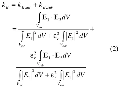
air and at the substrate. Therefore, Eqn. (1) can be expanded into

k_E = k_{E air}_, +k_{E sub}_,

∫

ε +

⋅ ε

+ ε

+ ⋅

=

sub air

sub

sub air

air

V r V

V r

V r V

V

dV E dV

E

dV dV E dV

E

dV

2 1 2 2

1 2

2 1 2 2

1

2 1

E E

(2)

where Vair and Vsub are the volume of the air and substrate, respectively, and kE,air is the electric coupling coefficient due to the air region and kE,sub is the electric coupling coefficient due to the substrate region.

(a)

(b)

Figure 2 Electric coupling structure of square loop resonators, (a) top view (b) side view of the coupling area. (Yeo, 2000)

3. Magnetic Coupling:

[image:3.595.324.526.149.295.2] [image:3.595.71.292.175.632.2]

(4)

103

stored energy of an uncoupled single resonator (Hong, 1996). This definition can be represented by

k dV H dV M V V = − ⋅

∫

H₁ H₂

1

2 (3)

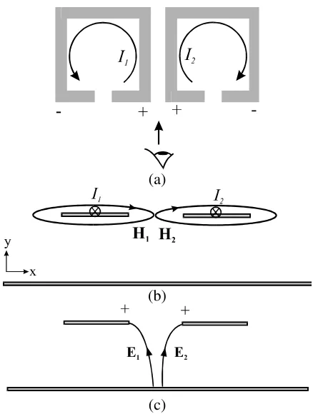
where H is the vector magnetic field. A negative sign is added in this equation to make it consistence with the electric coupling. The negative sign shows that the magnetic coupling has an opposite effect to the electric coupling when the structures are identical. When the two square loop resonators arranged symmetrically along the coupling plane as shown in Fig. 3(a), the magnetic coupling coefficient is negative. This is due to the x-component of magnetic fields, H1x and H2x, as shown in Fig. 3(b), are in same direction. The y-component of the magnetic field can be ignored in this argument because the y-component is very much weaker compared to the x-component. Therefore, the dot product of the two magnetic fields is positive which implied that the coupling coefficient is negative. A negative coupling coefficient is 180° out-of-phase with a positive coupling coefficient. Therefore, the electric and magnetic couplings are 180° out-of-phase when coupled through a symmetrical plane.

The magnetic coupling can also be divided into air and substrate region. Eqn. (3) can be rewritten as

k_M =k_{M air}_, +k_{M sub}_,

= − ⋅ − ⋅

∫

H H₁ ₂dV H₁ H₂

H dV dV H dV V V V V air sub 1 2 1

2 (4)

For non-magnetic substrate, the relative permeability,

µ

, is unity for both the air and the substrate. Therefore,

µ

is cancelled out in the top and bottom of the equation, which mean Eqn. (3) revert to (4).

(a)

(b)

Figure 3 Magnetic coupling structure of square loop resonators, (a) top view (b) side view of the coupling area. (Yeo, 2000)

4. Mixed Coupling:

Mixed coupling is defined as the superposition of electric coupling and magnetic coupling. For microstrip resonators, the mixed coupling coefficient can be written as

M E mix k k

k = +

∫

⋅ − ε + ⋅ ε + ⋅ = V V V r V V r V dV H dV dV E dV E dV dV sub air sub air 2 1 2 1 2 2 1 2 2 1 2 1 2

1 E E E H H

E

[image:4.595.308.525.187.419.2]

(5)

104

The mixed coupling can be divided into two types, namely the Type-I mixed coupling and the Type-II mixed coupling depending on the coupled field distribution.

4.1. Type-I Mixed Coupling:

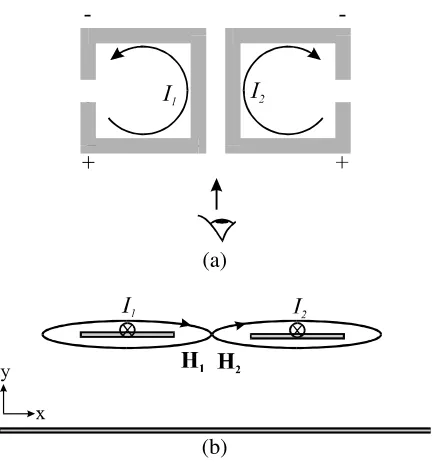
The Type-I mixed coupling occurs when the resonators are arranged asymmetrically along the coupling plane (i.e. resonator 2 is 180° rotation of resonator 1). This can be illustrated using square loop resonators as shown in Fig. 4. The x-component of magnetic fields, H1x and H2x, are in the opposite direction because the currents, I1 and I2, are flowing in opposite direction. Again the y-component of the magnetic field is very much weaker compared to the x-component in a microstrip structure. Therefore, the y-component can be ignored. Hence, the dot product of the magnetic fields, H1 and H2, is negative.

(a)

(b)

(c)

Figure 4 Type-I mixed coupling structure of square loop resonators, (a) top view. Side view of the coupling arms (b) the magnetic field (c) the electric field. (Yeo, 2000)

Even though the resonators are not a mirror image of each other, the coupled electric energy is still positive. This is because both the coupling arms of the resonators remain positive but different in magnitude. Therefore, the direction of electric fields, E1 and E2, is in the same direction as shown in Fig. 4(c). Since the dot product of electric fields is positive and the dot product of magnetic fields is negative, the electric and magnetic couplings are in-phase and enhancing each other. Note that the original definition of the mixed coupling assumed that the electric and magnetic couplings are out-of-phase.

In summary, the Type-I mixed coupling occurs when the electric coupling and the magnetic coupling are in-phase and coexist in the same coupling structure. Therefore, the electric coupling and the magnetic coupling are enhancing each other.

4.2. Type-II Mixed Coupling:

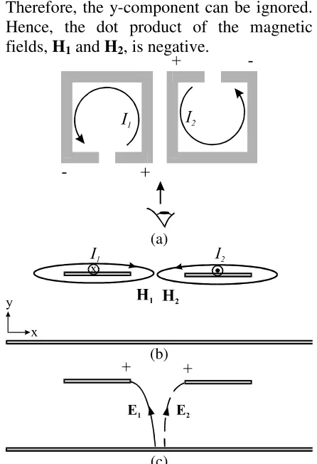
The Type-II mixed coupling occurs when the resonators are coupled through a symmetrical plane. This can be illustrated using square-loop resonators as shown in Fig. 5. The x-component magnetic fields,

H1x and H2x, are in the same direction because the currents, I1 and I2, are flowing in same direction. Therefore, the magnetic coupling is negative. The electric fields, E1 and E2, in this coupling structure are also in the same direction. Therefore, the electric coupling is positive. As a result, the electric and magnetic couplings tend to cancel out each other.

[image:5.595.68.291.373.699.2]

(6)

105

electric coupling and the magnetic coupling are out-of-phase and coexist in the coupling structure. Therefore, the electric coupling and the magnetic coupling cancel out each other.

Because of the cancelling effect, two different scenarios will be expected in the Type-II mixed coupling depending on the strength of the electric and magnetic couplings that coexists. This will be explained as follows:

4.2.1. Case 1. This case happens when the

resonators are very closely coupled; the electric coupling is stronger than the magnetic coupling. Because of the fact that the electric coupling decay at a faster rate compared to the magnetic coupling, a very special phenomenon occurs in this case.

(a)

(b)

(c)

Figure 5 Type-II mixed coupling structure of square loop resonators, (a) top view. Side view of the coupling arms (b) with magnetic field (c) electric field. (Yeo, 2000)

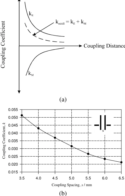
Fig. 6(a) shows the electric and magnetic couplings. The coupling coefficient is not always decreasing with increases coupling distance as expected in electric, magnetic and Type-I mixed coupling. The Type-II mixed coupling strength will decrease with increasing coupling distance until it reaches zero. Further increasing the coupling distance will result in the Type-II mixed coupling strength to increase with an opposite sign (negative). Fig. 6(a) shows a typical coupling coefficient curve of a Type-II mixed coupling.

(a)

Spacing, s / mm

0.2 0.7 1.2 1.7 2.2 2.7 3.2 3.7 4.2 4.7

C

o

u

p

li

n

g

C

o

ef

fi

ci

en

t,

kmix

II

*

-0.015 -0.010 -0.005 0.000 0.005 0.010 0.015 0.020 0.025 0.030

Section I Section II Section III

** Electric Coupling is defined as positive and Magnetic Coupling is defined as negative.

Electric Coupling = Magnetic Coupling

In

cr

ea

si

n

g

E

le

ct

ri

c

C

o

u

p

li

n

g

In

cr

ea

si

n

g

M

ag

n

et

ic

C

o

u

p

li

n

g

(b)

[image:6.595.307.526.277.710.2] [image:6.595.70.289.379.669.2]

(7)

106

When the coupling distance is very small between resonators the electric coupling is dominant. Therefore the coupling coefficient is positive. When the coupling distance is very far apart the magnetic coupling is dominant which is indicated with a negative coupling coefficient. The Type-II mixed coupling strength is zero at do, as shown in Fig. 6(a). This indicates that the electric and magnetic coupling totally cancel out each other at do. The phase of the Type-II mixed coupling will change after do indicating that the magnetic coupling is now dominant. The Type-II mixed coupling strength will increase after do until it reaches a second maximum coupling, kmaxII, at the coupling distance d1. Further increasing the coupling distance will reduce the Type-II mixed coupling strength again. This happens when the electric coupling in negligible small compared to the magnetic coupling.

Fig. 6(b) shows a practical example of this case. These coupling coefficients are obtained from full EM simulation of square loop resonators. All the behaviours described in Fig 5(b) are shown in the example. Microstrip hairpin topology (Hong, 1998) is also another example that experiences the case 1 of the Type-II mixed coupling.

4.2.1. Case 2. This case happens when the

resonators are very closely coupled; the magnetic coupling is very strong compared to the electric coupling.

Therefore, the Type-II mixed coupling is always dominated by the magnetic coupling as shown in Fig. 7(a). There is no change of phase in the Type-II mixed coupling in this case. The coupling coefficient is similar to electric, magnetic and Type-I mixed couplings because it decreases with the increasing of the coupling distance.

A practical example of this case is the forward coupled (Liang, 1994, 1995 &

Zhang, 1995), half wavelength resonators. Both peak charge density and surface current density are coexisted within the coupling volume of the forward coupled structure. Therefore, the forward coupled is a mixed coupling. Because the coupling plane is a symmetrical plane, the forward coupled is classified as Type-II mixed coupling.

(a)

Coupling Spacing, s / mm

3.5 4.0 4.5 5.0 5.5 6.0 6.5

C

o

u

p

li

n

g

C

o

ef

fi

ci

en

t,

k

0.015 0.020 0.025 0.030 0.035 0.040 0.045 0.050 0.055

(b)

Figure 7 Case 2, Type-II mixed coupling coefficients; (a) a typical coupling graph (b) a forward coupled coupling graph.

[image:7.595.309.520.252.583.2]

(8)

107

Therefore, it can be concluded that the magnetic and electric couplings in the parallel-aligned stripline resonators are equal. When the top dielectric of the stripline is removed to form microstrip, the electric coupling in the structure reduces. The magnetic coupling remains the same because it is independent of the relative permittivity. Therefore, the magnetic coupling in the parallel-aligned microstrip resonators (forward coupled resonators) is approximately twice stronger than the electric coupling.

Fig. 7(b) shows the plot of coupling coefficient against coupling distance for the forward coupled resonators. It is shown that the forward coupled exhibits the behaviour of the case 2, Type-II mixed coupling.

5. Numerical Example:

The scenarios discusses in the previous sections are assumed the resonators are designed to 50Ω line-width. However, changing the line-width will change the strength of the electric and magnetic fields. Fig. 8 shows two coupled resonators with their line-width increased. By increasing the line-width of the resonators, the charge density at the open end of the resonators is reduced. Therefore, this structure no longer produces pure electric coupling but, instead, the Type-II mixed coupling.

dx 6.6mm

1.2mm

Input _Output

1.8mm

5

.2

m

2

.5

m

2

.5

m

Figure 8 Two coupled square-loop resonators with increased line-width.

A numerical computation is also performed using Eqns. (2), (4) and (5) to determine the coupling coefficient. The electric and magnetic fields of the resonator are determined using a 3-D EM field simulator (Micro-Stripes). The coupling coefficients of the same structure are also computed using conventional method. For the conventional method, the two resonant modes of the coupled structure are simulated using EM Sonnet and the coupling coefficients are determined using (Hong, 1998)

2 1 2 2

f f

f f kc

+ −

= (6)

where f1 and f2 are the two resonant modes of the coupled structure. A plot of comparison between the numerical results and the conventional method is shown in Fig. 9. The results show good agreement between the numerical and the convention method for determining the coupling coefficients.

dx in mm

1.0 1.5 2.0 2.5 3.0 3.5 4.0 4.5 5.0 5.5 6.0 6.5 7.0 7.5 8.0

Kc

x

1

0

-4

-10 -5 0 5 10 15 20 25 30

Conventional Numerical

[image:8.595.309.520.420.649.2] [image:8.595.83.278.573.704.2]

(9)

108

6. Discussion and Conclusion:

All the discussion in Section II to IV is assumed even mode operation. The explanation is still hold true if the mode of operation is an odd mode. However, all the signs will change from positive to negative and vice-versa.

The authors have addressed the reason why the electric and magnetic couplings are out-of-phase when the resonators are arranged symmetrically along the coupling plane by purely looking at the coupled field distributions.

A detail discussion on Type-I and Type-II mixed coupling is presented. A structure can be classified as Type-I mixed coupling when the resonators are arranged asymmetrically along the coupling plane and Type-II mixed coupling when the resonators are arranged symmetrically along the coupling. We have also addressed the reason "why the electric and magnetic coupled energies enhance each other in the Type-I mixed coupling and cancel out each other in the Type-II mixed coupling?" through the coupled field distributions. A numerical computation of the coupling coefficients is also presented to further enhance this concept.

5. References:

Liang G. C., et. al., "High-Power HTS Microstrip Filters for Wireless Communication," IEEE MTT-S Intl.

Microwave Symp. Digest, pp. 183-186, 1994

Liang G.-C., et. al., "Power High-Temperature Superconducting Microstrip Filters For Cellular Base-Station Application," IEEE Trans. Appl. Supercond., vol. 5, 1995

Liang G.-C., et. al., "High-Power HTS Microstrip Filters for Wireless

Communication," IEEE Trans. Microwave

Theory and Tech., vol. MTT-43, No.12,

1995, pp. 3020-3029,

Hong J. S., Lancaster M. J., "Couplings of Microstrip Square Open-Loop Resonators for Cross-Coupled Planar Microwave Filters,"

IEEE Trans. Microwave Theory and Tech., vol. 44, 1996, pp. 2099-2109

Hong J. S., Lancaster M. J., "Cross-Coupled Microstrip Hairpin-Resonator Filters," IEEE Trans. Microwave Theory and Tech., vol. 46, 1998, pp. 118-122

Jokela K. T., "Narrow-Band Stripline or Microstrip Filters with Transmission Zeros at Real and Imaginary Frequencies," IEEE Trans. Microwave Theory and Tech., vol. MTT-28, 1980, pp. 542-547

Matthaei G. L., Hey-Shipton G. L., "Novel Staggered Resonator Array Superconducting 2.3-GHz Bandpass Filter," IEEE Trans. Microwave Theory and Tech., vol. 41, No.12, 1993, pp. 2345-2352

Yeo K. S. K., "High temperature superconducting microwave devices", Ph.D. Thesis, The University of Birmingham, 2000

Yeo K. S. K., Lancaster M. J., Hong J. S., "The Design of Microstrip Six Pole Quasi Elliptic Filter with Linear Phase Response using Extracted Pole Technique," IEEE

Trans. Microwave Theory and Tech, vol. 49,

No. 2, 2001, pp. 321-327

Zhang D., et. al., "Compact Forward-coupled Superconducting Microstrip Filters for Cellular Communication," IEEE Trans. Appl. Supercond., vol. 5, 1995