The Performance of RANS Models for Prediction of Flows in Meandering Channels

(1)

121

The Performance of RANS Models for Prediction of Flows in Meandering Channels

Usman Ghani1, Martin Marriott2, Peter Wormleaton3

1.

Assistant professor, Civil Engineering Department, UET Taxila, Pakistan

2

School of Architecture, Computing & Engineering, University of East London, UK

3.

Senior Lecturer, Department of Engineering, Queen Mary University of London, UK usman.ghani@uettaxila.edu.pk

Abstract: This research work presents the prediction capability of Reynolds Averaged Navior-Stoke,s equations based k-& k- turbulence models. Two solvers (SSIIM and FLUENT) were used in this research work. The performance of the two turbulence models was gauged for one flow case. Mesh dependency check was also done. Once it was proved that both the models produce approximately same results, the k- model was then tested for its suitability for studying various flow aspects of meandering channels. Two different meandering channel geometries with the same sinuosity (centre line planform geometry), main channel meander width/floodplain width ratio and same main channel aspect ratio were used. However main channel width varied in two cases. Both bankfull and overbank flows were considered. The bend radius to main channel width ratio (r/bc) of the wider main channel was

1.0 whereas it was 1.8 for narrow channel. The model predicted the depth averaged velocities (DAV), water surface profiles, velocity vectors in planforms at different levels with good accuracy. It captured all the salient features of the flow for inbank, low overbank and high overbank flows. From this study it can be concluded that k- model can be used with confidence in these types of meandering channels.

[Usman Ghani, Martin Marriott, Peter Wormleaton. The Performance of RANS Models for Prediction of Flows in Meandering Channels.Life Sci J 2013;10(10s):121-132] (ISSN:1097-8135). http://www.lifesciencesite.com. 20

Keywords: Meandering channel; overbank flows; turbulence model; Navior-Stokes equations.

1. Introduction

River flows are very complex even if the geometry of the channel is very simple such as a straight rectangular cross-section. This is mainly due to the fact that water flow is three dimensional and is derived from the combined action of a number of forces such as centrifugal forces, pressure driven forces, gravity forces and also shear forces due to transfer of momentum at the main channel floodplain interaction layers.

Flow behaviour in rivers is very important for river engineers because it is closely related to river flood prediction, warning and alleviation schemes as well as for the overall planning of river and floodplain management. It has its importance in navigation, water intakes, evolution of river bed and sediment transport. Due to all of these factors research into compound meandering channels is of much practical importance and engineering application. Research into two stage meandering compound channels has been carried out for the last three decades. This research included different approaches such as theoretical, laboratory or field observations and numerical techniques using computers.

In straight channels the secondary flows are generated due to turbulence anisotropy. The turbulence anisotropy is caused due to the presence of free surface and walls. The free surface and walls reduce the turbulence intensity normal to the surface

which is then redistributed in other directions resulting in turbulence anisotropy. Due to the existence of this anisotropy in straight channels, the standard k-or k-turbulence models which are based on Boussinesq,s assumption does not capture the secondary circulations in these channels.

However in the case of meandering channels this turbulence anisotropy is weaker as compared to pressure and shear driven cells. The imbalance between shear driven secondary cells and centrifugal forces generated pressure driven cells are the main cause of secondary cells in meandering compound channels (Ervine et al. 1993, Wormleaton et al., 2004, Myers et al, 2000).

(2)

122 impact of turbulence closure models used in the simulation has also been investigated in different CFD studies.

As stated above, due to weak turbulent anisotropy driven secondary cells, in this research work the k- model has been investigated for its suitability in meandering channel simulations. In the past some researchers used a finite volume based 3D model SSIIM (Olsen, 2011) for this case. They used the k- turbulence model with a structured mesh. However the same model can be used with an unstructured mesh generally consisting of triangular elements. It can also be used in k- form. In order to determine the relative performance of the different meshes a structured mesh using SSIIM was compared with a triangular mesh using FLUENT; both models using the RANS k- model. The results were also generated with SSIIM using the k- model with an identical structured grid. The models were compared with each other and with Marriott’s, 2007, experimental data from a compound meandering channel with a rectangular cross section. These data comprised of two main channel widths both having the same aspect ratio, sinuosity and main channel meander width/floodplain width ratio.

2. The Experimental Investigation

The experimental data used in this work has been obtained from Marriott’s work at the University of Hertfordshire (Marriott, 1998). Two different meandering channel geometries with the same

sinuosity (centre line planform geometry), main channel meander width/floodplain width ratio and same main channel aspect ratio were used. However main channel width varied in two cases. Both bankfull and overbank flows were considered. The bend radius to main channel width ratio (r/bc) of the

wider main channel was 1.0 whereas it was 1.8 for narrow channel.

Three different bed slopes with two different overbank flow depths were considered for each geometry. The planform consisted of a meandering rectangular main channel made up of centre line circular arcs with a radius of 500 mm and included angle of 140 degrees joined tangentially at the cross over points. The resulting sinuosity was 1.3 for both the geometries. The important dimensions of the channels and floodplains along with 3D view of the channel are as shown in Fig. 1 and Table 1. Different experimental runs reported in this paper have been named by three digits. The first digit stands for geometry (1 for wide geometry and 2 for narrow geometry), the second for bed slope (1 for low, 2 for intermediate and 3 for steep slope) and the third one for bankfull and overbank flow depths ( 0 for bankfull, 1 for low overbank and 2 for high overbank). Thus case number MJM1 111 means wide geometry with low slope and low overbank flow depth. Table 1 shows various geometric parameters of the channels.

(3)

123

[image:3.612.96.514.73.271.2]

Planform 2 – Narrow Channel

Figure 1. Geometry of the experimental channels Table 1 – Leading channel/floodplain dimensions

Dimensions (lengths in mm) Wide Channel Narrow Channel Main Channel

Width (bc) (mm) 507 282

Depth (hc) (mm) 115 63

Aspect Ratio 4.57:1 4.48:1

Sinuosity 1.3 1.3

rc/bc 1.0 1.8

Floodplain

Width (Bf) (mm) 1230 1016

Meander belt width (Bm) (mm) 1158 938

Bm/Bf 0.94 0.92

3. The Numerical Model

3.1. Governing Equations

The governing equations for the models used in this paper are continuity and Reynolds-averaged Navier-Stokes equations (RANS). For steady state incompressible flow, the RANS equations can be written in Cartesian coordinates as (Patankar, 1980)

Continuity equation

0   

i i

x U

Momentum equation





1 )

( i i j

i i

j

j i

j

j F uu

x P x

U

x U x U

x

U   

       

  

     

  



 



The terms in these equations are as follows.

P

is the pressure,



and



are the kinematic viscosity and density of the water respectively,

U

_iis the time-averaged velocity component in

x

_i direction,

F

_i denotes external force (gravity forces), and

u

_i

u

_j are the Reynolds stresses which result from the decomposition of instantaneous velocities into their mean and fluctuating components. In these models the Reynolds stresses are expressed using the Boussinesq relationship as below.

ij i

j

j i t j

i

k

U

v

u



3

2 























(4)

124 respectively. For the k- model, transport equations are derived for the turbulent kinetic energy, k, and the rate of viscous dissipation, . These are then solved and used to calculate the eddy viscosity in above equation as



_t



C

_

k

2



, where C is a constant in the model which takes a standard value of 0.09. The k- model utilizes transport equations for k and the turbulence frequency







k

from which

can be determined.

In all cases a logarithmic wall law for rough boundaries was used to determine near-wall velocity. This is written as:

_

     

 

s b k

y u

U 30

ln 1

*

U is the velocity at a distance yb from the

boundary, u* is the shear velocity, ks is an equivalent

particle diameter for the bed material and  is the von Karman constant (0.4). The near-wall values of k and  are taken as:





c u k

2 *

and

b y u

  

3 *

The equivalent particle diameters for each run were calculated from Marriott’s measured values of Manning’s n using Strickler’s formula

A “rigid lid” assumption, which prescribes a surface that is usually planar was taken as a boundary condition for the free surface (That is water surface was defined as a plane of symmetry). At the plane of symmetry, normal gradients of all the variables and normal velocity were set as zero except the rate of dissipation. The pressure on the surface was not set at zero but represents the variation in the water depth

that would occur if the surface was not fixed. Thus a pressure greater than zero represents super elevation and a pressure less than zero represents surface depression. No slip wall boundary condition was taken at bed and side walls.

3.2. Grid Design and Dependence

A structured grid covering four meander wavelengths was adopted for the SSIIM modelling. Each wavelength was modelled using 40 x-increments. There were 40 lateral y-increments divided equally between the channel and floodplains. The main channel depth was modelled using twelve depth z-increments. The meandering channel geometry was created by blocking out the bottom seven of these increments in order to create the floodplains. The size of the lateral floodplain increments increased geometrically from the main channel interface to the outer floodplain edge. Thus the increments were small in the high shear main channel/floodplain interface region so as to capture the relatively rapid local flow variations.

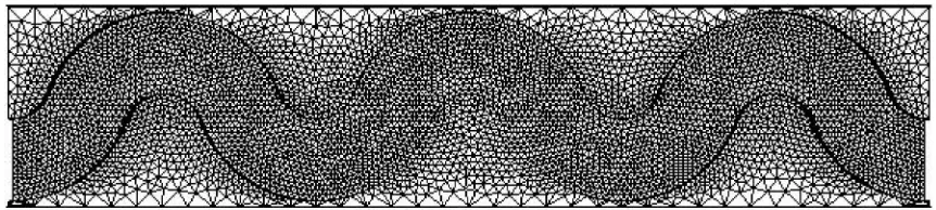
[image:4.612.88.519.515.612.2]

An unstructured tetrahedral mesh was used to discretize the geometry for simulation using FLUENT. The mesh used had the following node numbers 201×15×10 in the longitudinal, lateral and vertical directions respectively in the main channel. Since flow parameters within and close to the channel boundaries show the greatest local variation, the mesh was made fine in these areas and gradually coarsened on the floodplain away from the main channel. As a result a mesh of 201×36×6 was used in the floodplain. The lateral grid sizes on the floodplains decreased gradually from the outer floodplain edge to the main channel bank. The final mesh used for simulation in FLUENT has been shown in Fig.2.

Figure 2. The unstructured FLUENT mesh

A post processing check on mesh quality based on assessing the skewness of the generated mesh elements indicated that the mesh is of high quality and would not compromise solution stability. The solutions at successive meander apices were compared in all the models and the differences were sufficiently small to assume with confidence that

flow parameters within the observed meander were unaffected by inlet or outlet conditions.

4. Results and Discussion 4.1. Model Comparisons

(5)

125 with those obtained by doubling the number of x, y and z nodes. The mean absolute error (MAE) as a percentage of the velocities in the x, y and z directions were 1.9%, 2.9% and 4.3% respectively. These were thought to be acceptably small bearing in mind the accuracy of the measured data.

The FLUENT model improved the overall percentage MAE for primary velocities in run 111 by 0.3% over the SSIIM solutions. In view of probable interpolation and numerical computational errors, this difference was accepted by the Authors as additional confirmation of the grid independence of both models.

It is well known that the k- model tends to under-estimate the extent of separation and re-circulation at curved walls due to its tendency to over-predict the magnitude of turbulent shear stresses in these regions. The k- model on the other hand gives less turbulent diffusion than the k- model (Olsen, 2011) and so may be better suited to these regions. The Authors compared the performance of the SSIIM k- and k- models for inank run 110. It was found that the k- model was faster and more robust, i.e. allowed the use of larger relaxation factors, than the k- method. It was observed that

over the whole meander the k- model was 1% better in terms of the percentage MAE for primary velocities than the k- model. However the k-

model was 1.7% better in the cross-over sections where the re-circulation was greatest. In areas of no re-circulation the difference in the models was less than 0.5%. Both models under-predicted the extent of the re-circulation zone.

4.2. Bankfull Runs

The variation in depth averaged primary velocities for the in-bank runs in the two channel geometries are shown in Figure 3. It can be seen from Figure 3 that the calculated depth averaged primary velocities are very similar to the observed values for both channels at the apex showing maximum values near the inner side. However at the cross-overs the velocities at the inner side are over-predicted in both cases as discussed above.

Figure 4 shows the planform variation in velocities at 45mm above the bed. As reported by Marriott (1998 & 1999) and Wormleaton & Marriott (2007) separation and recirculation is observed downstream of the inner apex wall in the wide channel (run 110) but not in the narrow channel (run 210).

Run 110 - Apex

-0.1 0.0 0.1 0.2 0.3 0.4

0 100 200 300 400 500 Distance from LH Side (mm)

V

e

loci

ty

(

m/

s

)

Run 210 - Apex

0.0 0.1 0.2 0.3 0.4

V

e

lo

c

it

y

(

m

/s

)

(a) (b)

Figure 3(a-b). Depth averaged velocities for in-bank flows (square indicates observed and line shows calculated values of velocities)

Run 110 - Cross-Over

-0.1 0 0.1 0.2 0.3 0.4

V

el

oc

ity

(

m

/s)

0.0 0.1 0.2 0.3 0.4

V

elo

c

it

y

(

m

/s

)

3(c) 3(d)

[image:5.612.99.516.375.502.2] [image:5.612.97.515.537.668.2]

(6)

126

2 2.2 2.4 2.6 2.8 3 3.2 3.4 3.6 0.2

0.4 0.6 0.8 1

2 2.2 2.4 2.6 2.8 3 3.2 3.4 3.6 0.2

0.4 0.6 0.8 1

2 2.2 2.4 2.6 2.8 3 3.2 3.4 3.6 0.2

0.4 0.6 0.8

2 2.2 2.4 2.6 2.8 3 3.2 3.4 3.6

0.2 0.4 0.6 0.8

Note: All horizontal scales are distance downstream in metres All vertical scales are lateral distance in metres. Velocity scale 0.3m/s =

Observed Observed

Calculated Calculated

Wide Channel - Run 110 Narrow Channel - Run 210

Figure 4 - Planform velocity distributions for bankfull flows - Wide channel at 50mm above the bed and narrow channel at 45mm above the bed.

Bagnold (1960) stated that this separation occurs when the ratio of the channel centre-line radius (rc) to the channel width (bc) is less than 2. The

value of this ratio (rc/bc) is 1.0 for the wide channel

and 1.8 for the narrow channel. Thus the observed results broadly concur with Bagnold’s criterion. Flow separation would be expected in the wide channel whereas the narrow channel is in the marginal region and although re-circulation is not observed, the inner bank velocities downstream of the apex are very small. In Figure 5 the numerical model is seen to have computed the water surface variation generally within ±1mm of the observed values.

4.3. Over-Bank Runs

The observed and calculated discharges in the main channel below floodplain level are shown in Table 2 below. For geometry 1 it can be seen that the main channel discharge at the apex (Qca) is well

modelled except for run 121 where it is somewhat over-estimated. The source of this variation can be traced in more detail from Figures b. In Figure

6a-b it is apparent that the maximum velocity filament in all flows is near the inside bank at the apex. For the lower bed slope (i.e. lower velocities) in Figure 6a the calculated and observed depth averaged velocity (DAV) values at the apex are in close agreement. However at the higher bed slope it can be seen from Figure 6b that a region of lower DAV values is observed at around 150mm from the outer bank.

[image:6.612.93.513.77.379.2]

(7)

127 Run 110 - Apex

108 110 112 114 116

-300 -200 -100 0 100 200 300

Dist from Channel Centre-Line (mm)

W

a

te

r

Lev

e

l (

mm)

108 110 112 114 116

-300 -200 -100 0 100 200 300

Wat

e

r Lev

e

l

(m

[image:7.612.325.527.70.314.2]

m)

Figure 5. Water surface variations for inbank flow.

Run 210 - Apex

56 58 60 62

-200 -100 0 100 200

Dis t from Channel Centre-Line (mm)

Wat

er

Lev

el

(

m

)

56 58 60 62

-200 -100 0 100 200

W

a

ter

Le

ve

l

[image:7.612.82.276.73.314.2]

(mm)

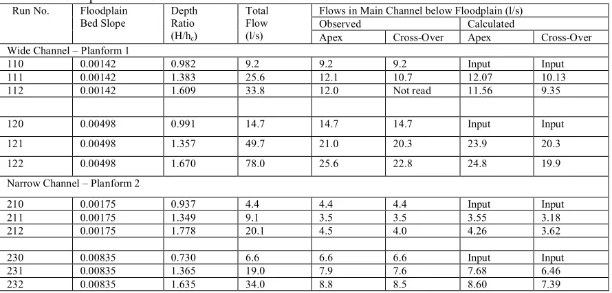
Table 2 – Comparison of Observed and Calculated Main Channel Flows

Run No. Floodplain Bed Slope

Depth Ratio (H/hc)

Total Flow (l/s)

Flows in Main Channel below Floodplain (l/s)

Observed Calculated

Apex Cross-Over Apex Cross-Over

Wide Channel – Planform 1

110 0.00142 0.982 9.2 9.2 9.2 Input Input

111 0.00142 1.383 25.6 12.1 10.7 12.07 10.13

112 0.00142 1.609 33.8 12.0 Not read 11.56 9.35

120 0.00498 0.991 14.7 14.7 14.7 Input Input

121 0.00498 1.357 49.7 21.0 20.3 23.9 20.3

122 0.00498 1.670 78.0 25.6 22.8 24.8 19.9

Narrow Channel – Planform 2

210 0.00175 0.937 4.4 4.4 4.4 Input Input

211 0.00175 1.349 9.1 3.5 3.5 3.55 3.18

212 0.00175 1.778 20.1 4.5 4.0 4.26 3.62

230 0.00835 0.730 6.6 6.6 6.6 Input Input

231 0.00835 1.365 19.0 7.9 7.6 7.68 6.46

232 0.00835 1.635 34.0 8.8 8.5 8.60 7.39

The cross-over DAV comparisons in Figure 6a indicate that the maximum velocity filament has moved across the channel from the inner bank at the apex to the outer bank at the cross-over, this is captured by the model. However at the higher bed slope in Figure 6b it is clear that the observed DAV values across the channel are more uniform laterally although the numerical model still gives higher DAV values at the outer bank. It is noticeable that the observed DAV at 100mm from the left hand for run

122 is lower than the adjacent points; this is not an error in reading and is repeated at other cross-over points. It is due to flow interference between the main channel and floodplain flows at the interface and results in the low DAV zone observed subsequently at the apex as discussed above.

[image:7.612.67.512.362.575.2]

(8)

in-128 bank to low over-bank the main channel component will generally decrease due to turbulent energy losses at the main channel floodplain interface. Indeed this behaviour is seen for the narrow main channel in

geometry 2. However, for geometry 1 the main channel component increases and this is due to the fact that in going over-bank the zone of re-circulation is removed.

Run 111 - Apex

0.0 0.1 0.1 0.2 0.2 0.3 0.3 0.4

0 100 200 300 400 500

Distance from LH Side (mm)

Vel

o

ci

ty

(m

/s)

0 0.1 0.2 0.3 0.4

0 100 200 300 400 500

V

el

o

ci

ty

(

m

/s)

6a(i) 6a(ii)

Run 112 - Apex

0 0.05 0.1 0.15 0.2 0.25 0.3 0.35

0 100 200 300 400 500

Dis tance from LH Side (mm)

Vel

o

ci

ty

(

m

/s)

6a(iii)

Run 121 - Apex

0 0.1 0.2 0.3 0.4 0.5 0.6 0.7

0 100 200 300 400 500

Dis tance from LH Side (mm)

V

el

o

ci

ty

(

m

/s

)

0 0.2 0.4 0.6 0.8

0 100 200 300 400 500

V

e

lo

ci

ty

(

m/

s)

6b(i) 6b(ii)

Run 122 - Apex

0.0 0.2 0.4 0.6 0.8

0 200 400

Ve

locit

y

(m/

s)

Run 122 - Cross Over

0.0 0.2 0.4 0.6 0.8

0 100 200 300 400 500

V

el

o

ci

ty

(

m

/s)

(9)

129 Run 211 - Apex

0.0 0.1 0.2 0.3 0.4

0 50 100 150 200 250

V

e

lo

c

it

y (

m/

s)

0.0 0.1 0.2 0.3 0.4

0 50 100 150 200 250

V

e

lo

c

it

y

(

m/

s)

6c(i) 6c(ii)

Run 212 - Apex

0.00 0.10 0.20 0.30 0.40

0 50 100 150 200 250

V

e

lo

ci

ty

(m/

s)

0 0.1 0.2 0.3 0.4

0 50 100 150 200 250

V

e

lo

c

it

y

(

m

/s)

6c(iii) 6c(iv)

Run 231 - Apex

0.00 0.10 0.20 0.30 0.40 0.50 0.60 0.70

0 50 100 150 200 250

Vel

oc

it

y (

m/

s)

0 0.2 0.4 0.6 0.8

0 50 100 150 200 250

V

e

lo

c

it

y

(

m

/s)

6d(i) 6d(ii)

Run 232 - Apex

0.00 0.10 0.20 0.30 0.40 0.50 0.60 0.70

0 50 100 150 200 250

V

e

lo

c

ity

(

m/

s)

0 0.2 0.4 0.6 0.8

0 50 100 150 200 250

Distance from LH Bank (mm)

V

e

lo

c

it

y

(

m/

s)

6d(iii) 6d(iv)

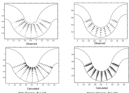
[image:9.612.68.491.76.573.2]

(10)

130 Note: All horizontal scales are distance downstream in metres All vertical scales are lateral distance in metres. Velocity scale 0.3m/s =

Observed Observed

Calculated Calculated

Wide Channel - Run 111 Narrow Channel - Run 211

2 2.2 2.4 2.6 2.8 3 3.2 3.4 3.6 0.2

0.4 0.6 0.8 1

2 2.2 2.4 2.6 2.8 3 3.2 3.4 3.6 0.2

0.4 0.6 0.8

2 2.2 2.4 2.6 2.8 3 3.2 3.4 3.6 0.2

0.4 0.6 0.8 2 2.2 2.4 2.6 2.8 3 3.2 3.4 3.6

[image:10.612.103.510.69.367.2]

0.2 0.4 0.6 0.8 1

Figure 7. Planform velocity distributions for overbank flows - wide channel at 50mm above the bed and narrow channel at 45mm above the bed.

154 156 158 160 162 164

-200 -100 0 100 200

Dist from C/L (mm)

Wat

e

r

L

ev

el

(

mm

)

Run 111 - Apex

154 156 158 160 162 164

-200 -100 0 100 200

Dist from C/L (mm)

Wat

er

Lev

e

l

(mm)

8(i) 8(ii)

145 150 155 160 165

-300 -200 -100 0 100 200 300

Dist from C/L (mm)

W

a

te

r Lev

e

l

(m

m)

Run 121 - Apex

145 150 155 160 165

-300 -200 -100 0 100 200 300

Dist from C/L (mm)

W

a

te

r

Le

v

e

l (

m

m)

(11)

131

180 185 190 195 200

-300 -200 -100 0 100 200 300

Dist from C/L (mm)

W

a

te

r

Le

v

el

(

mm

)

Run 122 - Apex

180 185 190 195 200

-300 -200 -100 0 100 200 300

Dist from C/L (mm)

W

a

te

r

Le

v

e

l (

mm)

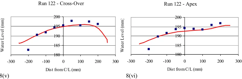
[image:11.612.73.486.72.207.2]

8(v) 8(vi)

Figure 8. Water surface variation for overbank flows It should be emphasised here that for the narrow channel geometry 2 only five lateral sets of readings were taken at 50mm spacing and at three depths of 20mm spacing. Thus there is some room for interpolation error between points and extrapolation error to the channel boundaries. Nevertheless it does appear that in general the apex flows are reasonably well modelled whereas the cross-over flows are underestimated. The geometry 2 DAV comparisons are shown in Figure 6c-d. It can be seen that the observed maximum DAV is again near the inside bank at the apices. The numerical model tends to over-estimate the maximum DAV for the lower bed slope as shown in Figure 6c and underestimate it at the higher flow and bed slope, run 232, as in Figure 6d. It is noticeable that the low velocity zone seen in the wider channel of geometry 1 does not occur in the narrower main channel. In fact a high velocity filament crosses from the outer bank at the upstream cross-over (-70o) to the inner bank halfway between the cross-over and the apex (-35o) where it remains until the next cross-over (70o). The numerical model captures this behaviour well leading to the relatively good predictions of discharge at the narrow main channel apices.

The cross-over discharges are underestimated increasingly with larger floodplain bed slope and depth of flow. In the experiments for the higher bed slope (231 and 232) surface standing waves were observed indicating flow at or near super-critical on the floodplain. This observation can be supported by considering the wide floodplain Froude numbers based upon Manning velocities. These are 0.69, 0.79, 1.66 and 1.82 for runs 211, 212, 231 and 232 respectively. At the cross-over points the floodplain flow crosses over the top of the main channel expanding as it enters the main channel and contracting as it leaves. If this process involves the transition from locally super-critical to sub-critical flow then a discontinuity (or standing wave) will occur. The numerical model handles such an abrupt

discontinuity by smoothing it out and this has indeed been observed in terms of calculated depth variations. The observed and calculated main channel depths for the steepest and deepest runs 231 and 232 are shown in Figure 8. The water surface levels in the numerical model agree well with observed values at the apex. However at the cross-over a standing wave some 12 mm high is observed and the numerical model simply smoothens this out. This may explain some of the relatively large discharge errors at the cross-overs, particularly since there is reasonable agreement between the observed and calculated DAV values as seen in Figure 6c-d.

5. Conclusions

In-bank and over-bank experimental data from a rectangular meandering channel at different bed slopes and flow depths have been modelled using a RANS k- and k- model. Two different main channel cross-sections have been used with the same aspect ratio and having meander planform of the same sinuosity. Two different RANS k- methods discretisation grids were checked against each other, a structured grid using SSIIM and an unstructured one using FLUENT. Both gave very similar results confirming the grid independence of the model.

In-bank flows in the wider main channel (geometry 1) produced a recirculation zone near the inner bank downstream of the apex; this did not occur in the narrower main channel (geometry 2). The RANS k- model captured this recirculation zone although not its full extent. The k- model gave very slightly improved results in the recirculation region although it was almost identical elsewhere. The k- model was shown to be faster and more robust, allowing larger relaxation factors. The in-bank water surface level variations were modelled satisfactorily.

(12)

132 the flow went over-bank. For geometry 2 the main-channel component initially decreased as the flow went over-bank, due to turbulent losses at the interface. The numerical model captured these different behaviours between the two geometries. The main-channel bulk discharge components for the over-bank flows at the apices were reasonably well predicted by the numerical model in all cases although those at the cross-overs were less so, particularly at higher depths and steeper bed slopes. This was thought to be due to the occurrence of standing waves on the floodplain caused by the floodplain flow crossing the main channel. The model tended to “smooth out” the discontinuities and rapid depth changes in these regions. The numerical model captured the general features of the observed data reasonably well. However it failed to capture a low velocity filament in the wide main channel which was created due to channel/floodplain interference at the upstream cross-over.

The simple k- model has been tested against over-bank experimental data covering a range of depths, bed slopes and channel/floodplain geometries. It has been shown to provide reasonably good agreement in depth averaged velocities in all cases. It also appears to capture most of the overall salient flow structures. The RANS k- model is one of the computationally fastest methods of modelling turbulent flows in open channel flows. It is particularly suited to meandering channels; both in-bank and over-in-bank, where the turbulent flows are largely geometry rather than boundary generated. As such it will be the method of choice in situations where the type/required accuracy of the output data, the channel geometry and the flow conditions permit. It is hoped that this paper will provide some guidance in identifying these conditions and limitations in the k- model when applied to meandering over-bank flows.

Acknowledgement:

The first author is highly acknowledged to Higher Education Commission Pakistan for the grant

provided to him to conduct this research work at Queen Mary University of London, UK.

Corresponding Author:

Dr. Usman Ghani Assistant Professor

Civil Engineering Department UET Taxila

E-mail: usman.ghani@uettaxila.edu.pk

References

1 Ervine DA, Willetts BB, Sellin RHJ, Lorena M. Factors affecting conveyance in meandering compound flows. Journal of Hydraulic Engineering 1993; 119(12): 1383-99.

2 Wormleaton PR, Sellin RHJ, Loveless JH, Bryant T, Hey RD, Catmur SE. (2004). Flow structures in a two-stage meandering channel with a mobile bed. Journal of Hydraulic Research 2004; 42(2): 145-62. 3 Myers WRC, Lyness JE, Cassells JB, O’Sullivan JJ.

Geometrical and roughness effects on compound channel resistance. Proc. I.C.E. Water Maritime & Energy London, 2000; 142(3): 157-66.

4 Wormleaton PR, Marriott MJ. An experimental and numerical study of the effects of width of meandering main channel on overbank flows. IAHR Congress Venice Italy 2007; 32: 575-82.

5 Wormleaton PR, Ewunetu M. Three dimensional k-ε numerical modelling of overbank flow in a mobile bed meandering channel with floodplains of different depth, roughness and planform. Journal of Hydraulic Research 2006;44(1): 18-32.

6 Olsen NRB. SSIIM Users’ Manual, The Norwegian University of Science and Technology, 2011. 7 Marriott MJ. The effect of overbank flow on the

conveyance of the inbank zone in meandering compound channels. IAHR Congress Graz Austria 1999; 28: 612-18.

8 Marriott, MJ. Hydrodynamics of flow around bends in meandering and compound channels. Ph.D thesis, University of Hertfordshire, UK,1998.

9 Patankar SV. Numerical heat transfer and fluid flow. McGraw-Hill, New York, 1980.

10 Bagnold RA. Some aspects of the shape of river meanders. US Geological Survey, Professional Paper 1960; 282E: 135-44.