Statistical inference for spatial and spatio temporal processes

(1)

STATISTICAL INFERENCE FOR

SPATIAL AND SPATIO-TEMPORAL

PROCESSES

A thesis subm itted to

the London School of Economics and Political Science

and the

University of London

in the subject of

Statistics

for the degree of

Doctor of Philosophy

(2)

UMI Number: U490B42

INFORMATION TO ALL U SE R S

The quality of this reproduction is d ep en d en t upon the quality of the copy subm itted.

In the unlikely even t that the author did not sen d a com plete m anuscript

and there are m issing p a g e s, th e se will be noted. Also, if material had to be rem oved, a note will indicate the deletion.

Dissertation Publishing

UMI U 490342

Published by ProQ uest LLC 2014. Copyright in the Dissertation held by the Author. Microform Edition © ProQ uest LLC.

All rights reserved. This work is protected against unauthorized copying under Title 17, United S ta tes C ode.

ProQ uest LLC

789 East E isenhow er Parkway P.O. Box 1346

(3)

S ig n e d d e c la r a tio n

I would like to declare th a t the work presented in this thesis is my own. Chrysoula Dimitriou-Fakalou

(4)

F

50

5

0

Library,

V

(5)

A b stract

First, the tim e series analysis was widely introduced and used in the statistical world. Next, the analysis of spatio-tem poral processes has followed, which is taking into account not only when, b u t also where the phenomenon under observation is taking place.

We m ainly focus on stationary processes th a t are assum ed to be taking place regularly over b oth tim e and space. We examine ways of estim ating th e param eters involved, w ithout the risk of coming up w ith a very large bias for our estim ators; the bias is the typical problem of estim ation for the param eters of stationary processes on Zd, for any

d > 2. We particularly study the cases of spatio-tem poral ARM A processes and spatial

auto-norm al form ulations on Z d. For b oth cases and any positive integer d, we propose estim ators th a t are consistent, asym ptotically unbiased and norm al, if certain conditions are satisfied.

(6)

C on ten ts

1 I n tr o d u c tio n 8

2 E le m e n ta r y r e su lts for p r o c e sse s o n a d -d im en sio n a l la ttic e 18

2.1 In tro d u c tio n ... 18

2.2 U nilateral orderings ... 19

2.3 Stationary p r o c e s s e s ... . 21

2.3.1 Linear p r o c e s s e s ... 22

2.3.2 Reverse s t a t i o n a r i t y ... 26

2.4 ARM A m o d e l s ... 31

2.4.1 Auto-Regressions and M o v in g -A v e ra g es... 34

2.5 A -dependent p r o c e s s e s ... 49

3 E s tim a tio n for A R M A m o d e ls o n a d -d im en sio n a l la ttic e 53 3.1 In tro d u c tio n ... 53

3.2 The problems of the A R M A ... 55

3.2.1 Unilaterality, causality and i n v e r t ib i li ty ... 55

3.2.2 Two sides of the e d g e -e ffe c t... 61

3.3 E stim ation for AR pro cesses... ... 65

3.3.1 Original Yule-Walker equations for the a u to -re g re ssio n ... . 65

3.3.2 M ethod of moments e s tim a to rs ... 66

3.3.3 Conditional likelihood e s tim a tio n ... 70

3.4 E stim ation for MA p ro c e s s e s ... 71

3.4.1 General Yule-Walker equations for the m o v in g -a v e ra g e ... 71

3.4.2 M ethod of moments e s tim a to rs ... 72

3.4.3 Modified likelihood,estim ation ... . 82

(7)

3.5.1 Introduction ... 99

3.5.2 Definitions ...100

3.5.3 E stim ators ... 103

3.5.4 Properties of e s ti m a t o r s ... 107

3.6 B ilateral ARMA m o d e l s ...127

3.7 Spatio-tem poral a u to -re g re s sio n s ... 136

3.7.1 O rder s e le c tio n ...138

3.7.2 Tests for linear m o d e ls ... 139

3.7.3 An application on d a ta recorded regularly in tim e and space . . . 141

4 S ta tis tic a l in feren ce for sp a tia l a u to -lin ea r sc h e m e s 150 4.1 In tro d u c tio n ... 150

4.2 Best linear p r e d i c to r s ... 152

4.3 Spatial auto-linear s c h e m e s ... 158

4.4 U nilateral and some bilateral au to -reg ressio n s... 159

4.5 E stim ation ... 164

4.5.1 Conditions ... 165

4.5.2 Conditional likelihood e s tim a to r s ... 168

4.5.3 Pseudo-likelihood and least squares e s t i m a t o r s ... 171

4.5.4 M ethod of moments e s tim a to rs ...176

4.6 Tests for spatial auto-linear s c h e m e s ... 183

4.6.1 Goodness of fit t e s t ... 183

4.6.2 Test for zero coefficients ... 184

4.7 A pplication on th e climate d a t a ...185

5 M o d e lin g d a ta o b serv ed irregu larly over sp a ce a n d reg u la rly in tim e 189 5.1 In tro d u c tio n ... 189

5.2 Spatial m o d e l in g ...191

5.2.1 Interpretation of the inverse covariance m atrix and best linear pre dictors 192

5.2.2 C om putation of the inverse covariance m atrix and the innovations a lg o r i t h m ... 197

5.3 Spatio-tem poral m o d e lin g ... 201

(8)

5.3.2 M ultivariate Time Series c o n t e x t ...202

5.3.3 Gaussian likelihood e s t i m a t o r s ... 204

5.4 Hypothesis t e s t i n g ...219

5.4.1 Tests for the serial d e p e n d e n c e ...219

5.4.2 Tests for the spatial in te rd ep e n d e n c e ... . 222

5.5 Forms of prediction and k r ig in g ...224

5.6 Mink and M uskrat spatio-tem poral d a t a ... 227

5.6.1 R estrictions on the p a ra m e te rs ... 230

5.6.2 Testing the interaction of mink and m uskrat ...232

6 E x a c t G a u ssia n lik elih o o d s for o b serv a tio n s from sp a tia l q u a rter A R M A m o d e ls 234 6.1 In tro d u c tio n ... 234

6.2 Linear-by-linear a u to -re g re s s io n s ...235

6.2.1 Gaussian lik e lih o o d s • • • 243 6.3 Q uarter m oving-averages... 244

6.3.1 First-order f i l t e r s ... ... . 244

6.3.2 S im u la tio n s ... 246

7 C o n clu sio n 256

A c k n o w led g em e n ts 262

(9)

List o f Figures

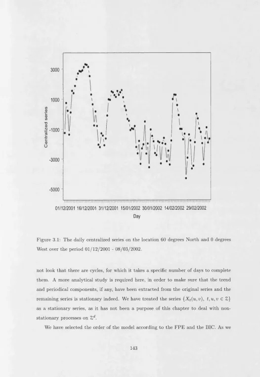
3.1 The daily centralized series on the location 60 degrees N orth and 0 degrees W est over th e period 01/12/2001 - 08/03/2002... 143

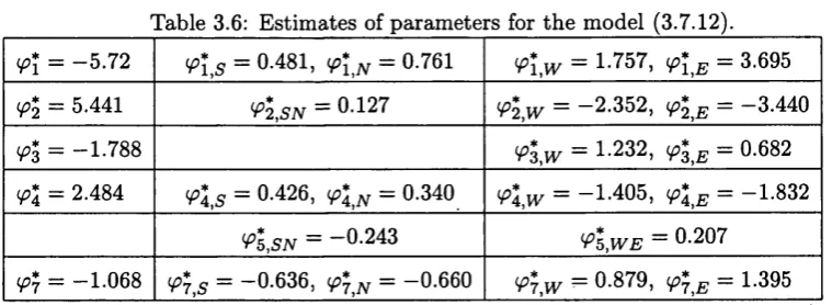
4.1 The centralized series on the 8th of March 2002 versus the ‘E ast-W est’ axis for the different latitudes of the ‘N orth-South’ axis...186

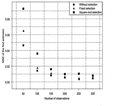
6.1 Absolute value of the bias of the estim ators a, a versus the num ber of observations from 100 replications...249

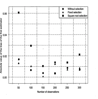
6.2 M ean Square E rror of the estim ators a, a versus the num ber of observa tions from 100 replications... 250 6.3 Absolute value of the bias of the estim ators 6, b versus the num ber of

observations from 100 replications...252 6.4 M ean Square Error of the estim ators b, b versus the num ber of observa

(10)

List o f Tables

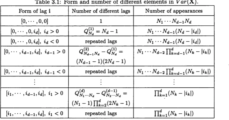
3.1 Form and num ber of different elements in Va r( X. )... 64 3.2 E stim ated Final Prediction Error for the five-nearest

neighbours model of order p... 144 3.3 BIC for th e five-nearest neighbours model of order p... 145 3.4 E stim ates of the param eters ipi,

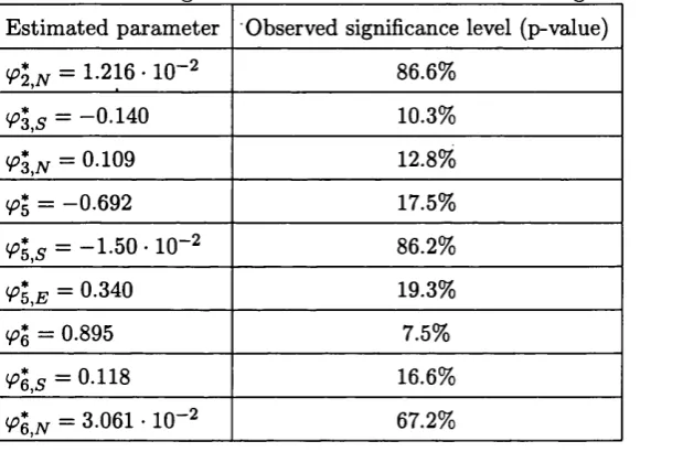
i = 1, • • • , 7, for the five-nearest neighbours model of order 7... 146 3.5 Insignificant results for the five-nearest neighbours model of order 7. . . . 146 3.6 E stim ates of param eters for th e model (3.7.12)...148

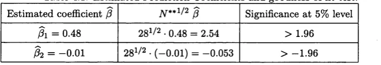
4.1 E stim ated Prediction Coefficients and goodness of fit te s t...188

(11)

Chapter 1

In trod u ction

Spatio-tem poral statistics is related to taking observations of a phenomenon at different tim es and different locations. It generalizes the notion of tim e series, by talcing into account the space where the phenomenon takes place too. This implies th a t, in addition to the tim e axis, a t least two more dimensions are added in th e analysis, depending on whether th e process takes place on the two or three-dimensional space. Thus, spatio- tem poral processes are an application of the processes th a t take place on a d-dimensional space or processes w ith d-dimensional indices, where d is any positive integer. Nowadays, the statistical analysis of spatio-tem poral processes has become very popular. It can be useful, for example, in geographical inform ation systems, in meteorology, in seismology, in physics or for environm ental applications over space and time.

(12)

Reverse strictly stationary processes are an example of a notion th a t has been in troduced particularly for spatial statistics. Like on the tim e axis there is the ‘p a st’ and ‘fu tu re’, each dimension of space also occupies two different ends. Nevertheless, there can be no causal relationship to relate those two ends. For example, the ‘p a s t’ and ‘fu tu re ’ of the tim e axis are such th a t there is a natural order between th e two, as anything th a t occurs in the ‘p a s t’ could have an effect on the happenings of th e ‘future’. The one dimensional spatial analogue of the tim e axis is the line transect, as this was described by W hittle (1954). For any two locations on the line transect, although those can be set in a unilateral order and they m ight be close enough to interact, there is usually no reason to assume th a t a causal relationship is taking place there.

In C hapters 3 and 4, we study the second-order properties of some (weakly) stationary processes th a t take place on the regular d-dimensional space. These processes might be spatial or spatio-tem poral; this depends on whether all the dimensions involved axe spatial, or w hether th e tim e axis is there as well. Studying their second-order properties is totally unconnected to the interpretation given to the d dimensions. Nevertheless, we will often refer to the inclusion or not of the tim e axis as a dimension, in order to study spatio-tem poral and spatial processes on Z d separately. For example, after we have defined the causal and invertible ARMA model on Z d in Section 2.4, we have proposed different ways for the estim ation of its param eters in C hapter 3. W hatever the number of dimensions d, an ARMA process on Z d is a standard way to model d a ta derived from a stationary process. Further as we axe going to see in Section 3.6, causal and invertible ARMA models, compared to all other ARMA models, provide more simplicity for the m ethods used. T he assum ption of causality and invertibility m ight be directly related to the presence of the tim e axis. Thus, spatio-tem poral ARMA models can often be better justified and understood th an spatial ARMA models, since when a directional preference m ust be assumed, it can be attrib u ted to th e unidirectional flow of the tim e axis only.

(13)

can be discovered in their spectral density, which has a finite, sym m etric and linear filter in the denom inator. Under the assum ption of normality, Besag (1974) expressed the second-order properties of the processes via a finite and linear conditional expectation of the value of the process on any location based on the values on all other locations of the lattice. W hen we m anage to mask the second-order properties of the process into a conditional expectation w ithout assuming th a t the process is Gaussian, then the process forms an auto-linear scheme. We will refer to such schemes as spatial auto-linear schemes, as including the tim e axis then would not be wise. This is because this form ulation does not distinguish between the information from the ‘p a s t’ and the inform ation from the ‘fu tu re ’, which should happen since, naturally, the inform ation from the ‘p a s t’ always comes first.

A t this point, it should be made clear th a t one of the purposes of this thesis is not to highlight the gap between the different m ethods of estim ation used for stationary spatial and spatio-tem poral processes b u t to bridge th a t gap instead. W hen it comes to estim ation, we try to establish in both C hapters 3 and 4, th a t any choice of param etrization for th e second-order properties of the process on Z d m ight be equally fruitful for the estim ators of the param eters. In other words, the estim ators we are proposing in the two chapters possess similar statistical properties. Thus, the reasons th a t make us consider C hapters 3 and 4 to be more related to spatio-tem poral and spatial processes, respectively, is prediction and not estim ation. For example, causal spatio-tem poral auto- regressions, such as these analyzed in Section 3.7, could be very useful for prediction, since the assumed model is only using locations from past timings. On the other hand, models th a t use all th e information around a location of interest, like the auto-linear schemes of C hapter 4, are more suitable for kriging (Cressie, 1993), which is the form of ‘spatial prediction’. Of course, it can be th a t we have the tim e axis in our analysis, th a t we are missing an observation from the centre of our d ataset and th a t we need to approxim ate its value. In this case known as smoothing, the param etrization adopted by an auto-linear form ulation m ight be useful for a tim e series or a spatio-tem poral process too.

(14)

as the num ber of dimensions increases, we cannot conclude yet th a t maximizing the exact Gaussian likelihood of observations can produce b o th asym ptotically unbiased and normal estim ators. This problem, which is reflected in the order of the bias of the estim ators, is known as the edge-effect and it has been very well described by Guyon (1982). T he source of the edge-effect is the different setting of asym ptotics th a t is taking place when d > 2. Indeed, although a set of observations on a finite set of Z d is available, usually a hyper-rectangle or hyper-cube, we should allow th a t this set could grow towards all sides. All the second-order stationary processes studied in C hapters 3 and 4, use this setting to assess the quality of the estim ators for the param eters of interest. Thus in both chapters, the estim ators must be defined in such ways, which guarantee th a t their asym ptotic norm ality can be established.

Defeating the edge-effect is one of the main challenges of this thesis. We have tried to tackle a very complex problem, for which the num ber of solutions proposed in the past has been lim ited. In C hapter 3, we have resorted to modifications of Gaussian likelihoods th a t may produce asym ptotically unbiased and norm al estim ators of the param eters. This is th e same tactic as the one followed by Guyon (1982) and Yao and Brockwell (2006), who referred to the estim ation of the param eters of any stationary process on Zd and the (p + q) param eters of two-dimensional causal and invertible ARMA processes, respectively. We have studied the cases of auto-regressions, moving-averages and ARMA processes on Zd, separately. Section 3.3 deals with causal auto-regressions and proposes a conditional Gaussian likelihood for maximization. By contrast, Section 3.4 is dedicated to invertible moving-averages only. There axe two new suggestions for estim ation of the param eters and the second one is based on a modification of a Gaussian conditional likelihood. The way we have dealt w ith the moving-average there, is only a special case of the more general solution proposed next for the ARMA. Thus, Section 3.5 generalizes the results of 3.4.3 for the param eters of a causal and invertible ARMA(p, q) process. W ith a finite fourth moment of the error sequence of interest, th e (p + q) modified G aussian likelihood estim ators defined then are consistent, asym ptotically unbiased and norm al and they are efficient if the process under observation is Gaussian.

(15)

modified Gaussian likelihood proposed for m aximization in 3.5.3 is only a special case of th e quantity th a t should have been maximized, in order to derive the estim ators of the param eters of a bilateral ARMA(p, q) process. The p a th we have followed there is due to W hittle (1954), who, for two-dimensional processes, achieved a transition from th e Gaussian likelihood of the observations from a finite bilateral auto-regression to the same likelihood expressed in term s of the param eters of the AR(oo) representation of the process. For bilateral ARMA models on Zd, we generalize his suggestion with a correction on the Gaussian likelihood, which affects its determ inistic p a rt only. This correction fixes the bias th a t the estim ators of the auto-regressive and moving-average param eters would have, unless the process was causal and invertible, respectively.

Under no circumstances should th a t bias be considered to have any relation to the edge-effect. W hile the bilaterality of an ARMA process m ight add to the bias of the estim ators even when d = 1, the edge-effect is very well disguised then, and makes its unpleasant appearance when d > 2, by causing the bias to move towards zero at equal

(d = 2) or slower (d > 2) speed, compared to the speed of the standard error of the

estim ators. It might fairly be considered as the most difficult problem to tackle regard ing th e estim ation of the param eters of a stationary process on Zd. This is the problem for which Guyon (1982) and Yao and Brockwell (2006) proposed solutions. Guyon used the form of Gaussian likelihood, which, according to W hittle (1954), involves the peri- odogram or sample auto-covariances in its random part. He corrected the edge-effect by using the unbiased estim ators of theoretical auto-covariances there. On the other hand, Yao and Brockwell (2006) focused on two-dimensional ARMA models. Before m odifying the genuine Gaussian likelihood, they used the innovations algorithm and a conventional unilateral ordering of locations in the sample; next they factorized the de term inant involved into a product of prediction variances in th e determ inistic part, and they partitioned the random p a rt into a sum of squares of prediction errors. Then, they p u t forward a selection of locations out of the ones available in the sample, and they used this inform ation only in the product and sum of the determ inistic and random part, respectively, of the proposed modified Gaussian likelihood.

In Section 3.5.3, we have suggested a new modification for a Gaussian likelihood, which is m ade especially for the ARMA on Z d. In other words, we have not restricted

our num ber of dimensions d to be small, like Yao and Brockwell (2006). We have tried to

(16)

using classical tim e dom ain argum ents, rather th an follow th e route of Guyon (1982). The special characteristics of the ARMA have been highlighted and taken into account. Yao and Brockwell (2006) resorted to the AR(oo) representation of the ARMA process of interest; as a result, they introduced an infinite order to their problem and missed the opportunity to generalize their results to higher dimensionalities. Similarly, Guyon’s (1982) suggestion would dem and the com putation of as m any sample auto-covariances as possible, unless the ARMA was a finite auto-regression or a finite moving-average. We have tried to dem onstrate th a t the ARMA deserves a solution, which takes into account its finite order. The finite order reflects b o th th e finite auto-regressive and moving-average polynomials. Indeed, an Auto-Regressive Moving-Average can become a moving-average, if a finite linear transform ation is applied to it. B ut w hat are these special advantages of these two characteristics, i.e. th a t the transform ation used is finite and th a t th e transform ed process is a moving-average?

On th e one hand, the finite transform ation implies th a t, for any set of random vari ables from the ARMA of large enough cardinality, we may create a set of smaller cardinal ity of random variables from the moving-average and ‘nothing is m issing’, i.e. information on more locations from the ARMA process could only contribute by offering more lo cations available from the moving-average, but not by augm enting the inform ation on the sites already available, as we have everything we needed to know there. As the original set grows, so does its subset a t equal speed. T h a t is our first victory over the edge-effect, which clearly reflects the auto-regressive nature of the ARMA. Indeed, finite transform ations work for the auto-regression as they m ight produce a sequence of uncor related random variables or they might produce a moving-average. Section 3.3 deals with problems of estim ation for auto-regressions via transform ations to white noise sequences, while estim ating the param eters of an auto-regression using the moving-average p a th is a special case of Section 3.5. Special reference to the auto-regression transform ed to a moving-average will also be made in Section 4.5.2.

(17)

variables on two different sites, as more sites available cannot give any random variables th a t have non-zero auto-covariance with any member of th e selected smaller set. Again, the cardinalities of the two sets move at the same speed and this signifies the second and final victory over th e edge-effect, thanks to the moving-average nature of the ARMA.

To use correctly these two properties, we have proceeded w ith modifications on Gaus sian likelihoods, rath er th an use them in their genuine form. As a result, the exponential functions of the modified likelihoods do not necessarily involve negative powers, and we cannot be sure th a t they can reach a minimum zero. This is a similar problem to the one th a t Guyon’s (1982) proposed estim ators had, as they were based on sample auto covariances th a t did not necessarily have a positive-definite sample variance-covariance m atrix or positive spectral estim ates, as those last ones were to be computed for the likelihood version of W hittle (1954). Dahlhaus and Kiinsch (1987) dealt successfully w ith this problem by introducing ‘d a ta tap e rs’, b u t paid the price of losing the efficiency of estim ators for d > 4. Such corrections on our proposed estim ators are beyond the in terests of this thesis. It is remarkable th a t this problem does not concern the estim ators of Yao and Brockwell (2006), as they make sure th a t a positive quantity is always to be m inimized, involving a sum of squares of prediction errors.

Since m ost of our attem pts to estim ate the param eters of ARMA models are counted on Gaussian likelihoods and modifications made on them , we retu rn to this subject again in C hapter 6 and examine it from a different scope. We focus there on two-dimensional ARM A processes only, although our results might be generalized when d > 2. First, for a special class of causal auto-regressions, which are linear-by-linear (M artin, 1979), we are able to write down explicitly the exact Gaussian likelihood of observations on a rectangle. In C hapter 3, we have only dealt w ith modifications on Gaussian likelihoods, but now the exact Gaussian likelihood version can be w ritten down, if such an auto-regression provides a sensible representation of the second-order properties th a t are being studied. Then, for observations from an invertible moving-average, which uses two param eters only, since we cannot write the exact Gaussian likelihood then, we perform simulations to w atch th e performance of the exact Gaussian likelihood estim ators and compare it to th a t of the modified estim ators proposed by Yao and Brockwell (2006). We are trying to conclude if its w orth to proceed w ith modifications when th e dimensionality of the problem is still low.

(18)

m ethod of estim ation for the unknown coefficients involved. It is a m ethod based on the m om ents of a new series, which may be produced from the original series, if a finite and linear filter is applied. This property, i.e. th a t w ith a finite transform ation we may produce a series w ith an auto-covariance function which cuts off to zero outside a finite set of vector lags, sounds like the property of an auto-regression th a t can be transform ed into a moving-average. Indeed, in Section 4.4, we show th a t, especially in term s of second-order properties rath er th an conditional expectations, it is always possible for an auto-regression to have an auto-linear representation. This same property of the auto regression was used in C hapter 3 as a main tool against the edge-effect. Using th a t same tool, we have studied the spatial auto-linear schemes of any dimensionality d, as we can always produce the new series w ith a finite transform ation.

(19)

auto-linear scheme. A complete result would involve b oth defining new estim ators and discovering their statistical properties.

It should be m ade clear now th a t both C hapters 3 and 4 try to model the second-order properties of (weakly) stationary processes on Zd\ either this is for a unilateral spatio- tem poral process or a spatial process on Zd, the same idea has been used repeatedly. In the end of Section 2.4.1, the subsection referring to the general Yule-Walker equations has given th e answer to alm ost all our questions, regarding the estim ation of param eters on Z d. T he general Yule-Walker equations relate the second-order properties, i.e. the auto-covariance functions, of two processes. Moreover from a stationary process, it is always possible to apply a linear, ‘tim e’-, or otherwise, invariant filter, in order to come up w ith a new stationary process, th a t is such th a t the two processes share together the general Yule-Walker representations. The filter one has to apply is none other than the one w ith coefficients equal to the auto-covariances of the second process th a t is about to be produced. As a result, if one of the two processes has the advantage of a finite num ber of non-zero auto-covariances, then all one has to do is apply a finite linear filter on th e other process to use this advantage. E ither we are dealing w ith an auto-regression or an ARM A or even a stationary process th a t has an auto-linear representation, a finite transform ation will autom atically make it a moving-average, or, in general, a process with similar second-order advantages. The question why these ideas were not th a t necessary and useful for processes th a t take place on Z, can only lead us to one answer. It is the edge-effect th a t has m ade us look for finite filters to apply on d a ta and finite auto covariance functions to assume for the processes of interest. It is the edge-effect th a t has m ade us resort to the general Yule-Walker equations, instead of the standard techniques used for tim e series.

Finally, in C hapter 5 we have changed the general setting followed so far, for the analysis of stationary processes on Zd, and we have switched to spatio-tem poral processes on Jld and Z, respectively. It is a very common problem th a t the locations where the phenom enon is taking place might be anywhere. In those cases the inclusion of the tim e axis in the analysis m ight have a worthless contribution. More specifically, we follow the statistical analysis of observations recorded on any N locations of R d and regularly over tim e. This is because, unless we record observations regularly over space, we cannot use any of theoretical background th a t has been studied in C hapters 3 and 4. We consider an

(20)

over time. Next, using a m ultivariate tim e series setting and allowing for the num ber of regular recordings over tim e to tend to infinity, we fit m ultivariate auto-regressions and use a conditional Gaussian likelihood, in order to estim ate the unknown spatial and tim e param eters and to assess the quality of our estim ators.

(21)

Chapter 2

E lem en tary results for processes

on a d-dim ensional la ttice

2.1

In tr o d u ctio n

Before we move to the next two chapters th a t deal w ith some problems of statistical inference for processes on the regular d-dimensional lattice and before we propose various ways to solve them , we will need to summarize some basic definitions and results th a t have been given before, as well as to add some new results th a t will be extremely useful next. In Section 2.2, we recall the notion of unilateral ordering between any two locations v T, v T + j T e Zd, which was given by W hittle (1954) when d = 2 and by Guyon (1982) when d > 2. Section 2.3 defines the weakly and strictly stationary processes and states the Wold decomposition, which provides a link between (weakly) stationary processes and linear processes. In th a t same section, we prove some properties of processes, which are linear functions of independent and identically distributed random variables. A new definition of the so-called reverse strict stationarity might also be found there, which is an a tte m p t to extend the definition of strict stationarity in a way th a t does not favor any direction of each one of the d dimensions. Later in Proposition 2.5 and, consequently, in C hapter 3 and Sections 4.4 and 4.5, we have used conditions, which are satisfied if the process of interest is reverse strictly stationary. Thus, when we establish in the end of Section 2.3.2 th a t reverse strictly stationary processes exist, a t the same tim e we allow for some of our conditions used in C hapters 3 and for 4 to be more realistic.

(22)

d-dimensional lattice and study their second-order properties. We focus on the special case of auto-regressions and moving-averages th a t not only share the same polynomial, b u t also they are generated by the same sequences of uncorrelated random variables. W hat we call the general Yule-Walker equations follow next, which provide a link be tween the auto-covariance functions of an auto-regression and a moving-average with the same polynomial. These equations will be further used in C hapter 3, which will only deal w ith ARMA processes, b ut they will also be used in C hapter 4. This is because they refer to the second-order properties of two processes, rath er th an any causal formulation considered to be taking place there. Not only will these equations be used as the theo retical base for a m ethod of moments suggested in Sections 3.4.1 and 3.4.2, b u t also they are the key used, in order to find the forms of inverse conditional variance m atrices for a set of random variables either from the auto-regression or th e moving-average process of interest and m ainly for Gaussian processes. Later in C hapter 3, this will allow us to use these m atrices in Gaussian conditional likelihoods. Again, since the derivation of these m atrices is based on the general Yule-Walker equations, we will also use these results to w rite conditional likelihoods in C hapter 4, even though the random variables there, m ight not have been generated from an auto-regression or a moving-average. We conclude the chapter w ith Section 2.5, in order to come up w ith a central limit theorem for processes on the regular d-dimensional lattice.

2.2

U n ila te r a l orderings

We consider ( X (v ), v r e Z d} to be a real valued process, where d is a positive integer and v = [ui, • • • , Vd] is a d-dimensional vector index. We denote w ith > the lexicographic order on Z d; when d = 1 this is the same as the standard order on Z. W hen d = 2, the notion of unilateral ordering was defined by W hittle (1954). For the general case of any positive integer d, we explain below the ordering due to Guyon (1982, p .96). We write

j = [ji, J2, • • • ,jd] > 0 = [0,0, • • • ,0]

on Z d, if

j i > 0

or

(23)

on Z d~l .

W hen d > 1, w riting j > 0 may have different meanings. For example, for two- dimensional processes

\j1J2] > [0,0]

if

h > 0

or

j i = 0 and j 2 > 0,

as described before. B ut we could also change the order of th e indices and write

\j2J 1] > [0,0]

if

32 > 0

or

j 2 = 0 and j i > 0.

One interesting question would be how many such representations exist for general num ber of dimensions d. To answer th a t, we first consider th e d distinct dimensions w ith two different ends. For the tim e axis, these would be th e ‘p a s t’ and the ‘future’ and would have a n atu ral order. It could also be the ‘w est’ and ‘e a st’ or the ‘south’ and ‘n o rth ’ for th e dimensions of space. Next, we define an hierarchy between the dimensions indicated by the labels k = 1, • • • , d. The m ost im portant dimension is labelled as 1 and the least im p o rtan t one as d. Dimension fc = 1, • • • , d — 1, is considered more im portant th an dimension k* = k -1- 1, • • • ,d, when moving its index towards any side has the same effect on the ordering of two locations, regardless of the way the other index has changed. For example, moving from tim e 1 and location labelled as 2 to either tim e 2 and location 3 or tim e 2 and location 1, is considered as moving to the future since tim e is going forwards in b o th cases. In general, there are d\ ways to label the different dimensions and the tim e axis is usually considered the most im portant of all and it is labelled as dimension 1.

(24)

each dimension k = 1, • • • , d, and there are 2d ways altogether. For example, for d = 2 we can define 22 = 4 different orderings. Say there is the dimension ‘west-east’ first and the dimension ‘south-north’; the 4 representations can be labelled as ‘w est-south’ and ‘east-n o rth ’ or ‘w est-north’ and ‘east-south’. Of these, 2d~1 choices can be seen as the counterparts of the rem aining 2d~l representations. For example, ‘east-north’ is the counterpart of ‘w est-south’, since it corresponds to the opposite quarter of Z 2. Similarly, ‘east-south’ is the counterpart of ‘w est-north’.

2.3

S ta tio n a r y p rocesses

We extend the definitions of weak and strict stationarity for processes w ith d indices, where d is any positive integer.

D e f in itio n 2.1 (W e a k s ta t io n a r it y ) . (X (v ), v T € Z d} is a (weakly) stationary process if i?{ X2(v)} < oo, and

1. £?{X(v)} is a constant independent of v, and

2. C ov{X (v), X ( v + j)} is independent of v for every j T € Z d.

W ithout loss of generality, we will consider

£ { X (v )} = 0 (2.3.1)

unless stated otherwise. Then we will w rite the real-valued function

70)

= C o v { X ( v ) ,X ( v + j) } = £ { X ( v ) X ( v + j ) } (2.3.2)

to be the auto-covariance function of th e stationary process of interest defined for any lag j T £ Z d. This function is even in the sense th a t

70)

= 7 ( - j ) , j T

e

Under th e condition th a t 7(-) is an absolutely summable function, we define the spectral density of 7(-) to be

9{W) = ? 2 ^ S ^ ( j ) ’ “ T e I" * - < (2-3.3)

5Te z d

(25)

D e fin itio n 2.2 (S tr ic t sta tio n a r ity ). The process ( X ( v ), v T E Z d} is said to be strictly stationary if the joint distribution of [X (vi), • • • , J f ( v g)]T and

[X (v1+ j ) , - . . ,X ( v , + j)]T are the same for all positive integers q and for all v r . - - , v j , r e z d.

2.3.1 Linear p rocesses

We consider {u(v), v T E Z d} to be a white noise sequence of random variables when they are generated on the points of Zd and they are uncorrelated w ith each other. We may then state the Wold decomposition.

T h eo r e m 2.1 (W old d e c o m p o sitio n ). A zero-mean and (weakly) stationary process { X (v), v T E £ d} w ith spectral density p(-), such th a t

I log g(u)du) > —oo, (2.3.4)

J [—

can be expressed in the form

I ( v ) = w ( v ) + ^ ^ j u ( v - j ) , (2.3.5)

j>0

where

1- Ej>oV’| < 0 0 ,

2. (u ( v )} ~ W iV(0, cr2).

Finally, a 2 = exp{(27r)-d / [_7r 7r]d log/(u;)du>} is given by Kolmogorov’s formula, where

/(w ) = (27r)d • 0(w), u>T E [ -7r, 7r]d.

For the proof of the theorem, see Rosanov (1967, p.64) for d, = 1 and Helson and Lowdenslager (1958) for d = 2, the proof being similar for d > 2 (Guyon, 1982, p.96).

(26)

Now th a t the Wold decomposition has been established, it is useful to derive the asym ptotic properties of linear processes for any d > 1 num ber of dimensions. Next, we prove two propositions th a t follow from Proposition 6.3.10 and Proposition 7.3.5 of Brockwell and Davis (1991).

P r o p o s it io n 2.1 (W e a k L aw o f L a rg e N u m b e r s fo r lin e a r p ro c e s s e s ). Let (L (v ), v r G Zd} be the linear process defined by

E l i j l c o o , { W ( v ) } ~ I I D { v . , a 2),

j>0 j>0

and <S C Z d be a set of cardinality N . Then as N —> oo, it holds th a t

Ln = J j E

vTe«s \j> o /

P r o o f . F irst note th a t

|£{L (v)}| < S|Z.(v)l = £ 7 |^ i j H ^ (v-j)| < T^(y - j ) |}

j>0 j>0

= $^|i||£|W (v-j)| = S|W(v)| 53 1^1 < °°’

j>0 j>0

and the series is well-defined in the sense of convergence in probability. For positive integer K, we define the set

M-K = { \ j i j 2 , - " ,jd]T : j i = 1, , K , jk = ±1, - - - , ± # , k = 2, ••• ,d } U

U {[o, J2, ■ • • ,jd]T • 32 = 1, • • * , K , jk = ± 1, • • ■, ± K , k = 3, • • • ,d} U • - U

U { [ 0 ,0 ,- -• J d]T : j d = l , - - , t f } U { [ 0 , - - - ,0]T}. (2.3.6)

T hen for any fixed K , as N —> oo,

y ™ = ^ E E E E h,

v Te«S j t € Mk Jt € Mk v tG<S

jTeA^A-since for fixed j T G M k , it holds th a t { W (v — j), v r G <S} are independent and identically distributed random variables. We also define the constants

»l( K ) =h h

j t &Mk

and

(27)

p

Then Y n k — * ^ l { K ) as AT —> oo and h l { K ) —* VL as K —» oo. We now only need to show th a t

Note th a t

lim lim s u p P (|L /v — Yn k\ > e) = 0, for any e > 0.

K - > o o N —k x)

p (\l n - y n k\ > c) = p ( | i y , L M - j f E E

V T <ES v T € S j T £ M K

= E ' j ^ ( v - j ) i > e )

v T€<S j>0 v T€ S j T£ M K

= p ( i ^ E E w - j ) i > < )

v r €«S i T£ M K , i >o

* i ^ E E I ' j i s i ^ v - j ) !

vr e5 j > 0

= ; E iy£F([l,---,l]-j)|,

6

J > 0

where the inequality is due to Chebychev. Then,

E \ h \ = E i ' j i = E - liji — o,

JTj ^ * ' k^ / j l 'ljk^ >K h + E L2bfcl>^

as K —► oo.

P r o p o s it io n 2.2. If (C (v ), v T 6 Zd}, {.D(v), v T E Zd} are two linear processes such th a t

c (y) = j ; ^ ( v - i ) , E N < c o .

i>0 i>0

D (v ) = ^ d , W ( v - i ) , ^ | d i | < o o , { W '( v ) } - J J £ > (0,<72),

i>0 i>0

then for a set «S C Z d of cardinality N and j > 0, it holds th a t

j j J 2 C '(v )C '(v + j) f ^ q c i + j J a 2 = Cov{C (v), C (v + j)},

v T€«S \ i>0

J

5Z C (v ) £ > ( v + j) ( S Cidi+ j ) = C o v f C ^ ^ C v + j ) }

v r €«S \ i > 0 /

as N —> oo.

(28)

j i = j j

J2 J 2 Ci

c i *w( V + j - n

v T€<S v Te 5 i> 0 i* > 0

= ^ E E ' i q + j l V f v - i f + y j^ , VT€ 5 i > 0

where

^

S S Ci Ci*

W(v-i)W(v+j-i*)

VT€<S •. i* > 0 , i* # i + j

= ^ 2 ci ci* f ^ " 1 E w ( v - i ) w ( v + j - i * ) )

l, i* > 0 , \ v TG 5 /

For the first term 1Zvt g«S E i > o « c>+j W (v — ^ holds th a t (W ( v ) 2, v T G Z} are independent and identically distributed w ith mean cr2, and since ^ |q C|+j| < oo, from

i > 0

the Weak Law of Large Numbers for the linear process L j(v) = c’\ ci+j W ( v — i)2, it

i > 0

holds th a t

jj

D

(x> ci+j) sw v)!t = (Hci

v r G<S \ i > 0 / \ i > 0

i c i + j I >

as N —> oo.

It suffices to show th a t Yjjv — * 0. For i* ^ i + j, it holds th a t {W (v — i)W (v + j i*), v T G Z d} ~ WiV(0, cr4) and, hence,

Var f A T1 ^ ^ ( v - i)W (v + j - i*) J = A r V 0

\ v T<ES /

as IV —> 00. For M .k as defined in (2.3.6), we may define for fixed K

Yi N K = Y c>c>- f^ " 1 E ^ ( v - i W v + j - i * ) ) -£ + 0 ,

iT, i * T em k , \ v t g 5 /

iVi+J as TV —> 00. So,

- yjNJf I < B|W"[X,'-- , 1]W[1, ■ - - ,2]| ■

Y

W M +

Y

lcl l l cH +

Y

lCil lCl’ l I _>0’

r e M K , i *T & M K , r # M K ,i*T e M K , r , i * r ( M K ,

1*> 0, i> 0 , i* # i + j i, i* > 0 , i* # i + j

(29)

2.3.2 R ev erse sta tio n a rity

As we have seen in Definition 2.1, weak stationarity relates any two random variables of the process of interest and it ensures th a t their auto-covariance is a function of the d-dimensional vector difference of the two locations. Further, if the auto-covariance function depends on this vector through its norm only, the process is called isotropic. Isotropic processes allow for more specific considerations and they are beyond the scope of this thesis.

For th e definition of strict stationarity, we refer to any two random vectors and their distributions. The random vectors might be of any positive length, say q. In tim e series, strict stationarity means intuitively th a t the graphs over two tim e intervals of length q of a realization of th e process should exhibit similar statistical characteristics. B ut it does not m ean th a t those are the same characteristics as the ones exhibited within the same intervals if they are observed from future to past. For a process evolving on a line transect, as this was described by W hittle (1954, p.434), tim e is replaced by a dimension of space and this m ight not make sense. We may observe the process starting from any of th e two ends towards the other end. Thus, we wish to define a form of stationarity th a t means intuitively th a t the two graphs over the intervals of length q th a t sta rt from the same location, one from left to right and the other from right to left, exhibit similar statistical characteristics.

On th e other hand, when we deal with conditional probabilities in a tim e series, the n atu ral order of th e indexes plays an im portant role. For example, for the two random variables A ( l ) and A (2), we will rarely introduce in our analysis the conditional probabilities of X ( l ) given A (2), unless we are asked to. In this last case, we usually convert to these probabilities from the conditional probabilities of X ( 2 ) given X( l ) , using the Bayesian formula. The answer might come much faster if we know th a t the distribution of the random vector [X (l), X(2)]T is the same as the distribution of the random vector [X(2), X ( l) ] r , as this will imply both th a t the m arginal distributions of X ( l ) and X ( 2 ) are the same and th a t

P (X (1 ) = u\X{2) = v) = P { X ( 2) = u |X ( l) = v). (2.3.7)

(30)

According to Definition 2.2, for the general case of strictly stationary processes on the d-dimensional lattice, it holds for any j r E Z d th a t the two random vectors [X (v i), • • • , X (vq)]T and [ X ( v i + j ) , • • • , X ( v q+j ) ] T have th e same distribution, because

M

they refer to the same differences, i.e. v i — V2, • • • , v i — v q, • • • , v g_i — v q. As a

W

result, one can shift the random vector [A(vi), - • • ,A ( v g)]T a t any j T E Z d steps away, and the distributions of the new random vectors are still the same. B ut w hat if we are not interested in changing the location of the random vector b u t its direction? In other words, can we make sure th a t the random vector [ A( —vi ) , • • • , X ( —v q)]T has the same distribution as the random vector [ X( vi ) , -- - ,A ( v q)]T, although it refers to the differences of opposite sign, i.e. —v i 4- V2, • • • , —v i 4- v 9, • • • , —v 9_ i + v g?

D e f in itio n 2.3 (R e v e rs e s t r i c t s ta t io n a r it y ) . The process ( A ( v ), v T E £ d} is said to be reverse strictly stationary if the joint distribution of [X(j 4- vi ) , • • • , X (j 4- v g)]T and [X(j — vi ) , - - - , X ( j — v g)]T are the same for all positive integers q and for all

r , v j , - . - , V j e z * .

Now, it is clear th a t the differences between th e locations of the second random vector are all of opposite sign from the ones of the first vector, b u t th a t has no effect on its distribution compared to the distribution of the first random vector. The two vectors this tim e, b o th have to originate on the same location v T E Z d w ithout any shift. As a result, Definition 2.3 does not imply th a t for a reverse strictly stationary process ( A (v ), v T E &d}, the two random variables X ( v i ) and X ( v2) have the same m arginal distribution for any two locations v [ , V2 E Z d. For example, if d = 1 the random variables X ( —1) and A ( l ) have the same distribution since the two locations of interest are one step away from location 0. For the same reason, all the random variables

X { 2j 4 -1), j E Z, share th e same distribution and all the random variables X ( 2j ) , j E Z,

also share the same distribution, b u t the two distributions do not have to be the same. This is established in the next proposition, which relates the two forms of stationarity. We denote w ith O, £ the odd and even integer num ber spaces, respectively. We also denote w ith V any of the 2d orderings O d, £ x C?d-1, • • • , £ d.

P r o p o s it io n 2.3. Let (A (v ), v T E Z d} be a reverse strictly stationary process and define

(31)

T hen the process { X p (v ), v T E V } is strictly stationary.

P ro o f. Since the process is reverse strictly stationary, it holds for any positive integer q and any v [ , • • • , v g E Z d th a t the random vectors [X (v i), • • • , X ( v g)]T and

[X (—v i), • • • , X ( —v g)]r have the same distribution. This stems from Definition 2.3 when we set v = 0.

Similarly, it holds for any v T E Z d th a t the vectors [X(j — v i) , • • • , X (j — v g)]T and [ X(—j + v i), • • • , X (— j + v g)]T share the same distribution. On th e other hand and again from Definition 2.3, since the process is reverse strictly statio n ary the first of previous random vectors has the same distribution as [A(j + v i) ,- - - ,X ( j + v g)]r . The two argum ents combined together imply th a t the random vectors [X (v i — j), • • • , X(vg — j)]T and X ( v i + j ) , - - - , A '(vg+ j) ] r , or [-X'(vi), ■ - • ,X ( v g)]T and [X (v i + 2j), • • • ,X ( v g + 2j)]r share the same distribution for any j T, v j , • • • , v g E Z d. We can see th a t for any j*T E S d there is a unique element j T € Z d such th a t 2j = j* and, vice versa. T he proof is completed when we also see th a t for a specific E V, there is a unique elem ent + j*T E V for

any j*T E S d and vice versa. ■

Proposition 2.3 shows th a t the way a reverse strictly stationary process has been defined does not allow us to necessarily conclude th a t it is strictly stationary as well. As a result, we first require th a t a process is strictly stationary and then look for its ex tra attrib u tes. We may think of a simple example, where b o th properties exist and can be combined to derive useful results. We consider the case of a strictly and reverse strictly stationary process {X (v), v r E Z d}. Then the distribution of [X (v i), X { \ 2 ) Y is the same as th e distribution of [A (—v i), A ( —V2)]r , because of reverse strict stationarity, and this is the same as th e distribution of [X (—v i + v i + V2) , X ( —V2 + v i + V2)]r or [X (v2), X ( v i)] T, because of strict stationarity. In other words, we have reversed the order of the two locations v i and V2- It is fairly easy to show, for example, th a t this property holds for any pair of identically distributed (but not necessarily independent) Bernoulli random variables.

B ut is it possible to s ta rt from a strictly stationary process and show th a t it is reverse strictly stationary for any positive integer q? The following proposition gives a sufficient condition for a strictly stationary process to be reverse strictly stationary as well.

(32)

27*}, if th e joint probability function of [X (vi), ■ • ■ , X ( v g)]T is an even function of all the differences v i — V2, • • • , v 9_i — v g, for any positive integer q and v [ , • • • , v£ E Zd, then it is a reverse strictly stationary process.

P r o o f. Since the sequence is strictly stationary, we know th a t th e joint probability function depends on the possible differences of locations only. If we consider it an even function, in the sense th a t changing the sign of all differences results in the same distribution of the random vector on the new locations, then the sequence is reverse

strictly stationary. ■

The joint probability function of q random variables, say • • • , Xq, is such th a t its logarithm can be w ritten as

l og{Pxw ~,xq(xi, ■ • • , x q)} = K • gi{xi) + ^ X i • x j g i j( x i , X j ) + • ■ •

i i<j

+ x i ' - - x q g i t...)q( x i , - - - ,Xq)]. (2.3.8)

Besag (1974, p .197) claimed the existence of such functions gi(•),••• , <7i,...,g(-)> under some very mild conditions. He focused on the special cases where

\og{PX l ,...,xq(xi, • • • ,* ,) } = K • ( J ^ X i g i f a ) + ^ X i • x j fiij) (2.3.9)

i i<j

and called them auto-models. He then showed th a t = (3jj. Two examples are the

auto-logistic and the auto-norm al model. We will deal w ith the auto-m odels again in C hapter 4.

We let the strictly stationary sequence of random variables {X (v), v T E Zd} and any positive integer q. For fixed, v [ , • • • , v£ E Z d, we write for convenience

X (v j) = X iy i = 1, • • • , <?,

and the joint probability function of the vector [X (vi), • • • , X ( v g)]r denoted as P x i , - ,xq{xi, • • • >£g)- Then it should hold in (2.3.8) th a t

K = K { y i - v 2,--- ,v i - v q, - " ,v g_ i - v 9),

and th a t

9i(x) = g ^ \ x ) , « = 1, • • • , g,

and

(33)

and

9 l , ~ , q ( x i , " - , x q ) = g {q\ - V1 - V 2 , - - - , V i - V „ - - - , V ?_ i - V g , X l , - - - , X g ) ,

for some functions K(-), g ^ \ - ) , • • • , g ^ ( - ) - Reverse strict stationarity would require th a t these are even functions of the differences v i — V2, • • • , v i — v 9, • • • , v g_i — v q, as it is described in Proposition 2.4.

L em m a 2.1. A strictly stationary sequence of Gaussian random variables is reverse strictly stationary.

P ro o f. T he proof comes imm ediately from the fact th a t th e joint density of any q ( *

identically distributed Gaussian random variables is a function of the ]

auto-\ 2

covariances, i.e. an even function of all the possible differences.

R e m a r k 2.1. A part from the case of a Gaussian reverse strictly stationary process, as it was described in Lem ma 2.1, are there any other reverse strictly stationary sequences? We explain here how reverse strictly stationary processes can be produced and repro duced. We know th a t when we have a strictly stationary process ( X ( v ) , v T E Zd} and we apply for all v T E Z d the same linear filter, say

5 (v ) = S

h

* ( v - j ) >

i Tz z d j Te z d

then the new process {S '(v ), v T E Zd} is also strictly stationary. Similarly, if { X(v ), v T E

Zd} is reverse strictly stationary and we apply the sym m etric linear filter

R ( v ) = /0 X ( v ) + J 2 h [ * ( v - j ) + A ( v + j ) ] , ^ | Z j | < o o , (2.3.10)

j>0 j>0

(34)

Consider the simple case of the reverse strictly stationary process {X (v ), v r G 2,d} and the new process defined by the equation

R ( v ) = X ( v ) - M [ X ( v - j ) + X ( v + j ) ]

for some j T G Z d and IG 01. Then for any v T, j j G Z d, we m ay write the two-dimensional random vectors

X ( v )

X ( v - j L - j )

* ( v - j ) * ( v - j i ) * ( v - j l + j) * ( v + j )

and

X ( v )

^ ( v + j i + j ) X ( v + j ) ^ ( v + j l ) ^ ■ ( v + j i - j )

We can see im m ediately th a t the two vectors [i?(v),i?(v — ji) ] T and [ R ( v ) , R ( v + ji) ] T have the same distribution, since the random vectors [X (v ) , X (v — j i — j ), X (v — j ), X (v — j i ) , X ( v - j i + j ) , X ( v + j ) ] T and [ X ( v ) , X ( v + j i + j ) ,X ( v + j ) , X ( v + j i ) , X (v + j i - j), X ( v — j)]T have the same distribution too.

2 .4

A R M A m o d els

D e f in itio n 2.4. We define an ARMA process { Z ( v ) , v T G Z d} as

Z (v ) = ^ ( v - j ) + <r(v ) + e ( v - j ) , (e(v )} ~ W N ( 0,cr2), (2.4.1)

j € l p j € j q

where {6j, j G Xp} and {aj, j G J q} are the auto-regressive and moving-average coeffi

cients and b o th index sets Xp and J q are contained in the set {j > 0}. B oth the sets Xp and J q have finite cardinalities p and q, respectively.

R ( v )

1

I—

1

o o o

__

_

1

_ R ( v -f- j , ) _ ₁ o o o ₁

R(v) 1 0 I 0 0 I

(35)

For convenience, we introduce the vector back shift operator B = [Bi, • • • , B d], such th a t

B-*Z(v) = Z ( v - j ) , i r e z d.

This, of course, also implies th a t

B - 'Z ( v ) = Z ( v + j ) , j '6 Zi

For z = [zi, • • • ,Zd], we w rite z} = Ylt=i zk ■ We can then define th e polynomials

d d

&(z)= i - y i b jz j = 1 - 5 3 h n ^ and ° ( z ) = 1 + s ^ = 1 + s n z k

-j€lp j G2p fe=l jGkTq k =1

(2.4.2) Then model (2.4.1) can be w ritten as

6(B )Z (v ) = a (B )e (v ), {e(v)} ~ W N ( 0 , a2 ). (2.4.3)

For this, we have assumed th a t 6(z) and a(z) do not have common factors although they may still have common roots.

The process { Z ( v ) , v T e Z d} defined in (2.4.1) is causal if it adm its a purely MA representation

Z (v ) = e(v) + ^ 2 £(v “ j) (2-4 -4)

j>0

where E j>0 l^jl < oo. A causal { Z ( v ) , v T E Z} is always (weakly) stationary with m ean 0 and the auto-covariance function

° 2 {^j + E i> o V’iV’i+j} , j > 0

+ J = o (2 A 5 )

7 (-j)» j < 0

The lem m a below presents a sufficient condition for the causality. 7 (j) = E { Z { v + $)Z{v)} = <

L e m m a 2.2. The process defined in (2.4.1) is causal if

6(0, • • • , 0,0, z d) ^ 0 for all \zd\ < 1 and 6(0, • • • ,0, zd_ i, zd) ^ 0 for all \zd- i \ < 1

and \zd\ = 1 and • • • and 6(z) ^ 0 for all \z\\ < 1 and \zk\ = 1, k = 2, • • • , d,

(2.4.6)

where , z d E C, i.e. the complex num ber space. Furtherm ore, condition (2.4.6)

implies th a t the coefficients {^j} defined in (2.4.4) decay a t an exponential rate, and in particular

(36)

where a G ( 0 , l ) , C l > 0 are constants.

For the proof of the lemma, see Anderson and Ju ry (1974). Otherwise, we follow the same argum ent as Yao and Brockwell (2006) and the inequality (2.4.7) follows from the simple argum ent as follows. Let ip(z) = 1 -f V’j z^ where the coefficients V’j are

j>o

given in (2.4.4). Then ip(z) = a(z)/b(z). Due to the continuity of &(•), b(z) 7^ 0 for all z G Ss = {[zi, ■ • • , Zd] : 1 — S < \zk\ < 1 + J, k = 1, • • • , d} under the causality condition, where 5 > 0 is a constant. Thus, ip(-) is bounded on S s, i.e. | z^l < oo for any

j>o

z G Ss and, so a -h-'Hk=2\jk\ _* q as max { j i , \ jk \ } —► oo, where a G (0,1) is a k=2,- - ,d

constant.

R em a rk 2.2. (i) Inequality (2.4.7) also holds if we replace by its derivative with respect to 6j, j e J p, or aj, j G J q, under the condition (2.4.6). This can be justified via taking derivative on bo th sides of equation ip(z) — a ( z ) /6(z), followed by the same argum ent as above.

(ii) T he same condition guarantees th a t the auto-covariance function 7(-) decays at an exponential rate, i.e. 7(j) = 0 (aJ1+^ = 2 lJfcl), where a G (0,1) is a constant.

(iii) A partial derivative of 7(-) w ith respect to any of th e (p + q) param eters also decays at an exponential rate. This may be seen through combining (i) and the argument in (ii) together.

(iv) Condition (2.4.6) is not necessary for the causality when d = 2,3, • • •.

The process (Z (v ), v T G £} is invertible if it adm its a purely A R representation

Z ( v ) = E ( v ) + ^2<p5 Z ( v - } ) (2.4.8)

j>o

where E j>0 |<^j| < oo. Like in Lemma 2.2, one can write down a sufficient condition for the invertibility of an ARMA process.

L em m a 2.3. The process defined in (2.4.1) is invertible if

a (0, • • • , 0,0, Zd) ^ 0 for all

\z&\

< 1 and a (0, • • • ,0, z j - i , Zd) 7^ 0 for all |zd_i| < 1

and \zd\ = 1 and • • • and a(z) 7^ 0 for all \z\\ < 1 and \zk\ = 1, k = 2, • • • , d,

(2.4.9)

(37)

The spectral density of { Z ( v ) , v T G Zd} as defined in (2.3.3) is of the form

r2

9 ( u ) = * (27r)‘

a(eiw) 2

, u?T G [—7r ,7r] . (2.4.10)

b(eiM)

If (Z (v ), v T G £ d} is causal and invertible, the spectral density g(-) is bounded away from oo and 0, respectively (Guyon, 1982). Note th a t the condition th a t g(-) is bounded away from oo and 0 is equivalent to the condition th a t a(z) b(z) ^ 0 for all ■ ■ • , zd G C w ith |z\ | = 1221 = • • • = 12^| = 1. Under this condition (Z ’(v), v T G £ d} is a (weakly) stationary process.

R e m a r k 2.3. At this point, we may see how bounding the spectral density of any (weakly) stationary process away from oo and 0 may be very useful to make conclusions on the variance m atrix of a set of random variables from this process. We consider any set S C Z d w ith N different elements, where N is a finite num ber, and the random variables { X ( v ) , v r G 5 } from a (weakly) stationary process w ith a bounded spectral density. T hen for the (IV x 1) random vector X w ith elements the random variables at any order, th e variance m atrix Var{X} has all its eigenvalues also bounded away from oo and 0. For the case th a t d = 1 and a set of consecutive observations, the proof has been given by Proposition 4.5.3 of Brockwell and Davis (1991). For the case th a t d = 2 when the observations lie on a rectangle, we can find a similar proof in the paper by Yao and Brockwell (2006). For the general case of d num ber of dimensions and for any

v T, v * T G Z d and j = v — v* = [71, • • • , j d], it holds th a t j k G Z for all k = 1, • • • ,d. Then

it is

[ ei 'Zt=i“kjkdw1 ---dwd = f [ / eiUkjk<Ljk = 0 (2.4.11)

J\-n,ir]d k=1 J -k

if and only if at least one k = 1, • • • , d, is such th a t j k 7^ 0, or v ^ v*. As a result, one can follow the same sequel as Proposition 4.5.3 of Brockwell and Davis and prove th a t all the eigenvalues are bounded, even though the set <S may not have a specific structure on Z d.

2.4.1 A u to -R eg ressio n s and M oving-A verages

(38)

of the much simpler world of the auto-regression and the moving-average, as they both have desirable properties th a t can be used to solve these problems. Thus, we will need to look for auto-regressions and moving-averages in the ARMA, rath er th an attack it directly.

Moreover in this section, we are interested in dem onstrating various ways in which an auto-regression and a moving-average might be linked. A part from the obvious con nection th a t they m ay refer to the same polynomial, we are also interested in relating two such processes via the same white noise sequence of random variables. We then come up w ith results such as the general Yule-Walker equations, derived in th e last part of this section, which involve the auto-covariance functions of an auto-regression and a moving-average w ith the same polynomial. Those equations have been used as the theoretical prototypes th a t should be im itated by d a ta quantities to provide m ethod of moments estim ators in the next chapter.

For z = [z\, ■ • • , Zd] and 0 < j i < j2 < • • • < jq, we define the polynomial

0(z) = 1 + 0h zjl + • • • + 0U (2.4.12)

where th e coefficients are such th a t we can write

0(z) -1 = 1 + ^ 0 j z-i, ^ 2 |0 j| < oo. (2.4.13)

j>0 j>0

We first consider a w hite noise sequence (e(v)} ~ W N (0,1) which generates the moving-

average (Y (v ), v T € Zd}, such th a t

Y (v) = 0(B )e(v) (2.4.14)

and the auto-regression (A (v ), v T £ Zd}, such th a t

0 (B -1)X (v ) = e(v). (2.4.15)

If we define th e polynomial

7(z) = 0(z) 0(z~ 1) = J 2 7(j) zJ> (2.4.16)

p e r

th en from (2.4.14),(2.4.15) and (2.4.16), we can see imm ediately th a t

(39)

The set T C Z d in (2.4.16) has finite cardinality and is such th a t 0 T E T and th a t if

j T

E T then —

j T

E T , as well. More specifically, we can w rite here

^ =

{jT :j = jn, -jn, jn -jm ,

ra,m

= l,--- ,9}.

L ater in C hapters 3 and 4, we will denote by T other finite sets of lags th a t include the zero lag and they axe symmetric, but we will not know their exact elements then.

If we define the polynomial

c(z) = 7(z) -1 = 0(z) -1 ^ (z- 1) - 1 = c0 ) z j> S < °°> (2.4.18)

jTezd j r e z d

we can re-write (2.4.17) as

X (v ) = c(B )T (v ). (2.4.19)

As a counterpart to th e process defined by

e(v ) = X (v ) + 0ji X ( v

+ ji) +

• • • + 6iqX ( y +

j 9),

we define

li(v) = X (v ) +