University of East London Institutional Repository: http://roar.uel.ac.uk
This paper is made available online in accordance with publisher policies. Please scroll down to view the document itself. Please refer to the repository record for this item and our policy information available from the repository home page for further information.
To see the final version of this paper please visit the publisher’s website. Access to the published version may require a subscription.
Author(s): Palmer-Brown, Dominic; Lee, Sin Wee; Draganova, Chrisina; Kang, Miao.
Article title:Modal Learning Neural Networks Year of publication: 2009
Citation: Palmer-Brown, D. et al (2009), ‘Modal Learning Neural Networks’ WSEAS Transactions on Computers 8 (2) 222-236
Link to published version:
http://www.wseas.us/e-library/transactions/computers/2009/28-674.pdf
Modal Learning Neural Networks
DOMINIC PALMER-BROWN, SIN WEE LEE, CHRISINA DRAGANOVA, MIAO KANG School of Computing and Technology
University of East London,
University Way, London, E16 2RD UNITED KINGDOM
{ D.Palmer-brown, S.W.Lee, C.Draganova, M.Kang}@uel.ac.uk http://www.uel.ac.uk/cite
Abstract: This paper will explore the integration of learning modes into a single neural network structure in
which layers of neurons or individual neurons adopt different modes. There are several reasons to explore modal learning. One motivation is to overcome the inherent limitations of any given mode (for example some modes memorise specific features, others average across features, and both approaches may be relevant according to the circumstances); another is inspiration from neuroscience, cognitive science and human learning, where it is impossible to build a serious model without consideration of multiple modes; and a third reason is non-stationary input data, or time-variant learning objectives, where the required mode is a function of time. Two modal learning ideas are presented: The Snap-Drift Neural Network (SDNN) which toggles its learning between two modes, is incorporated into an on-line system to provide carefully targeted guidance and feedback to students; and an adaptive function neural network (ADFUNN), in which adaptation applies simultaneously to both the weights and the individual neuron activation functions. The combination of the two modal learning methods, in the form of Snap-drift ADaptive FUnction Neural Network (SADFUNN) is then applied to optical and pen-based recognition of handwritten digits with results that demonstrate the effectiveness of the approach.
Key-Words: - Modal Learning, Snap-drift, ADFUNN, SADFUNN, e-learning, Personalized Learning, Diagnostic Feedback, Multiple Choice Questions
1. Modal Learning Neural Networks
Twenty years ago there were already several forms of artificial neural network, each utilising a different form of learning. But at that time it was considered likely that one or at least a very small number of forms of learning would prevail and become ubiquitous. Along the way, many forms of learning, notably Back-propagation, Bayesian and Kernel methods have been hailed as superior forms. However, decades after the introduction of Kohonen learning, SOMs, and Backpropagation they are still being used alongside more recent methods such as Bayesian and SVM. No single method or mode prevails. A wide range of methods are still in use, simply because there are significant problems and datasets for which each method is suitable and effective.In this context, Modal learning arises from the desire to equip a single neural network or module with the power of several modes of
learning, to achieve learning results that no single mode could achieve, through exploitation of the complementary nature of each mode.
A mode is an adaptation method for learning that could be applied in more than one type of architecture or network. It is analogous to a human mode of learning, such learning by analogy or category learning. Modes of learning map onto NN learning objectives. Well known modes therefore include the Delta Rule, Backpropagation (BP), Learning Vector quantization (LVQ), and Hebbian Learning. In contrast The Adaptive Resonance Theory (ART) or Bayesian neural networks are more than a mode of learning, they define architectures and approaches to learning, within which particular modes are used.
minimal error), the learning agent’s objective function must be expressed differently in terms of the parameters of the learning machine (eg.
de/dw). Given the dislocation between the actual objectives of learning and the objective learning function of the learning agent, it is not possible to know a-priori which is the optimal learning mode to use.
For example, BP is good for approximation and transformation, but if the features within the data need to be assimilated (or memorised) directly, then learning vector quantization or SVM would be more appropriate. We are unlikely to know in advance. But the learning agent should be able to work out the most effective mode during, and as part of, the learning process.
Modal Learning (ML) contrasts with hybrid and modular approaches in which each module or network exhibits one mode, and modules are bolted together with each designed to solve a sub-problem. Limitations of one mode of learning per ensemble of neurons include the need for more neurons, layers or networks.
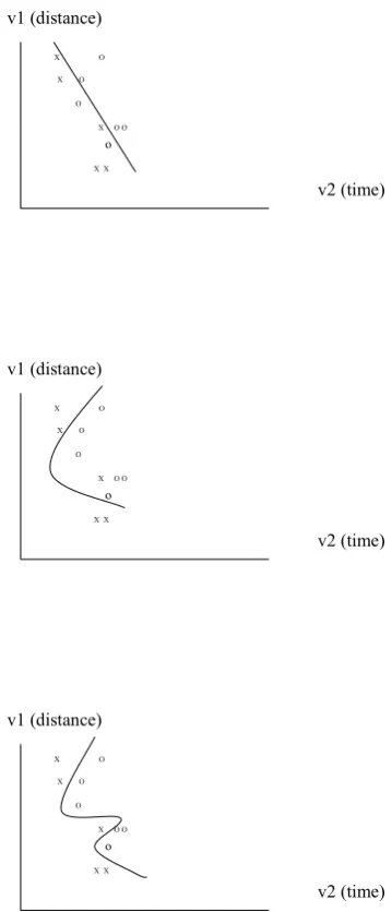
Even fixed task and data may benefit from sequential or simultaneous application of more than one mode, and data or task may be non-stationary. Each mode is inherently limited because it is tied to an objective function. A simple illustration of the potential benefits of a modal learning approach can be seen in the following sequence of class boundaries in a 2D, 2 class problem (Figure 1). In it we see how it is necessary to increase complexity to an extent that is not justified by the data in order to find a single mode solution.
Two Class Problem
v1 (distance)
X O
X O
O
X O O
o
X X
v2 (time)
v1 (distance)
X O
X O
O
X O O
o
X X
v2 (time)
v1 (distance)
X O
X O
O
X O O
o
X X
v2 (time)
v1 (distance)
X O
X O
O
X O O
o
X X
[image:3.595.327.507.115.534.2]v2 (time)
Figure 1: Increasingly complex solution to a
2-class problem
v1 (distance)
X O
X O
O
X O O
o
X X
v2 (time)
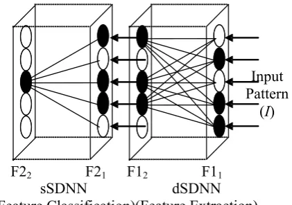
Figure 2: 3 mode solution
Or by combining a curve (multilayer percepton) and a cluster. This requires 2 modes of learning:
v1 (distance)
X O X O
O X O O
o
X X
v2 (time)
Figure 3: 2 mode solution
Rather than trying to solve the whole problem with a single mode of learning, a simpler learnt solution is achievable by combining modes of learning.
When we look at human and machine learning in a wider context, there are many reasons and motivations to consider modal learning, as it allows for the spectrum of learning to be taken into account, from memorisation to generalisation.
2. Snap-drift Neural Network (SDNN)
The snap-drift algorithm, which combines the two modes of learning (snap and drift) first emerged as an attempt to overcome the limitations of ART learning in non-stationary environments where self-organisation needs to take account of periodic or occasional performance feedback. Since then, thesnap-drift algorithm has proved invaluable for continuous learning in many applications.
The reinforcement versions [1], [2] of snap-drift are used in the classification of user requests in an active computer network simulation environment whereby the system is able to discover alternative solutions in response to varying performance requirements. The unsupervised snap-drift algorithm, without any form of reinforcement, has been used in the analysis and interpretation of data representing interactions between trainee network managers and a simulated network management system [3]. New patterns of the user behaviour were discovered.
Snap-drift in the form of a classifier [4] has been used in attempting to discover and recognize phrases extracted from Lancaster Parsed Corpus (LPC) [5]. Comparisons carried out between snap-drift and MLP with back-propagation, show that the former is faster and just as effective. It is also been used in Feature Discovery in Speech. Results show that the snap-drift Neural Network (SDNN) groups the phonetics speech input patterns meaningfully and extracts properties which are common to both non-stammering and stammering speech, as well as distinct features that are common within each of the utterance groups, thus supporting classification.
In most recent development, a supervised version of snap-drift has been used in grouping spatio-temporal variations associated with road traffic conditions. Results show that the SDNN used is bale to group read features such that they correspond to the road class travelled even under changing road traffic conditions.
the input layer F1, the distributed SDNN (dSDNN) will learn to group them according to their features using snap-drift [2]. The neurons whose weight prototypes result in them receiving the highest activations are adapted. Weights are normalised weights so that in effect only the angle of the weight vector is adapted, meaning that a recognised feature is based on a particular ratio of values, rather than absolute values. The output winning neurons from dSDNN act as input data to the selection SDNN (sSDNN) module for the purpose of feature grouping and this layer is also subject to snap-drift learning.
The learning process is unlike error minimisation and maximum likelihood methods in MLPs and other kinds of networks which perform optimization for classification or equivalents by for example pushing features in the direction that minimizes error, without any requirement for the feature to be statistically significant within the input data. In contrast, SDNN toggles its learning mode to find a rich set of features in the data and uses them to group the data into categories. Each weight vector is bounded by snap and drift: snapping gives the angle of the minimum values (on all dimensions) and drifting gives the average angle of the patterns grouped under the neuron. Snapping essentially provides an anchor vector pointing at the ‘bottom left hand corner’ of the pattern group for which the neuron wins. This represents a feature common to all the patterns in the group and gives a high probability of rapid (in terms of epochs) convergence (both snap and drift are convergent, but snap is faster). Drifting, which uses Learning Vector Quantization (LVQ), tilts the vector towards the centroid angle of the group and ensures that an average, generalised feature is included in the final vector. The angular range of the pattern-group membership depends on the proximity of neighbouring groups (natural competition), but can also be controlled by adjusting a threshold on the weighted sum of inputs to the neurons. The output winning neurons from dSDNN act as input data to the selection SDNN (sSDNN) module for the purpose of feature grouping and this layer is also subject to snap-drift learning.
3
E- learning Snap-Drift Neural
Network (ESDNN)
3.1 The ESDNN Architecture
In a recent application of snap-drift, ESDNN, the unsupervised version of the snap-drift
algorithm is deployed [6], as shown in Figure 4.
[image:5.595.329.540.175.323.2]
Figure 4: 1 E-learning SDNN architecture
During training, on presentation of an input pattern at the input layer, the dSDNN will learn to group the input patterns according to their general features. In this case, 5 F12 nodes,
whose weight prototypes best match the current input pattern, with the highest net input are used as the input data to the sSDNN module for feature classification.
In the sSDNN module, a quality assurance threshold is introduced. If the net input of a sSDNN node is above the threshold, the output node is accepted as the winner, otherwise a new uncommitted output node will be selected as the new winner and initialised with the current input pattern.
The following is a summary of the steps that occur in ESDNN:
Step 1: Initialise parameters: ( = 1, = 0) Step 2: For each epoch (t)
For each input pattern
Step 2.1: Find the D (D = 5) winning nodes at
F12 with the largest net input
Step 2.2: Weights of dSDNN adapted
according to the alternative learning procedure: (,) becomes Inverse(,) after every successive epoch
Step 2.3 Process the output pattern of F12 as
input pattern of F21
Input Pattern
(I)
F22 F21 F12 F11
dSDNN (
(Feature Classification) sSDNN
Step 2.4: Find the node at F22 with the largest
net input
Step 2.5: Test the threshold condition:
IF (the net input of the node is greater than the
threshold)
THEN
Weights of the sSDNN output node adapted according to the alternative learning procedure: (,) becomes Inverse(,) after every successive epoch
ELSE
An uncommitted sSDNN output node is selected and its weights are adapted according to the alternative learning procedure: (,) becomes Inverse(,) after every successive epoch
3.2 The ESDNN Learning Algorithm
The learning algorithm combines logical intersection learning (snap) and Learning Vector Quantisation (drift) (Kohonen, 1990). In general terms, the snap-drift algorithm can be stated as:
Snap-drift = (pattern intersection) + σ(LVQ) (1)
The top-down learning of both of the modules in the neural system is as follows:
wJi(new) = (I wJi(old)) + ( wJi(old) + (I - wJi(old))) (2)
where wJi = top-down weights vectors; I = binary input vectors, and = the drift speed constant = 0.1.
In successive learning epochs, the learning is toggled between the two modes of learning. When = 1, fast, minimalist (snap) learning is invoked, causing the top-down weights to reach their new asymptote on each input presentation. (2) is simplified as:
wJi(new) = I wJi(old) (3)
This learns sub-features of patterns. In contrast, when σ = 1, (2) simplifies to:
wJi(new) = wJi(old) + (I - wJi(old)) (4)
which causes a simple form of clustering at a speed determined by β.
The bottom-up learning of the neural system is a normalised version of the top-down learning:
wIJ(new) = wJi(new) /| wJi(new)| (5)
where wJi(new) = top-down weights of the network after learning.
In ESDNN, snap-drift is toggled between snap and drift on each successive epoch. The effect of this is to capture the strongest clusters (holistic features), sub-features, and combinations of the two.
4. E-learning System
4.1Motivation
Formative assessment provides students with feedback that highlights the areas for further study and indicates the degree of progress [7]. This type of feedback needs to be timely and frequent during the semester in order to really help the students in learning of a particular subject. One effective way to provide students with immediate and frequent feedback is by using Multiple Choice Questions (MCQs) set up as web-based formative assessments and given to students to complete after a lecture/tutorial session. MCQs can be designed with a purpose to provide diagnostic feedback, which identifies misconceptions or adequately understood areas of a given topic and explains the source of misconceptions by comparing with common mistakes. There are many studies (e.g. [8], [9], [10], [11], [12]) investigating the role different types of feedback and MCQs used in web-based assessments, that report on positive results from the use of MCQs in online tests for formative assessments. However none of these studies have employed any intelligent analysis of the students’ responses or providing diagnostic feedback in the online tests.
tool for self-assessment that is accessible anywhere and at anytime (eg. on the web).
The ESDNN is a simple tool that can be incorporated into a VLE system or installed on a PC, configured to run as a web server. The student responses are recorded in a database and can be used for monitoring the progress of the students and for identifying misunderstood concepts that can be addressed in following face-to-face sessions. The collected data can be also used to analyse how the feedback influences the learning of individual students and for retraining the neural network. Subsequently the content of the feedback can be improved. Once designed MCQs and feedbacks can be reused for subsequent cohorts of students.
4.2 E-Learning System Architecture
The E-learning system has been designed and built using the JavaServer Faces Technology (JSF), which is a component-based web application framework that enables rapid development. The JSF follows the Model-View-Controller (MVC) design pattern and its architecture defines clear separation of the user interface from the application data and logic. The ESDNN is integrated within the web application as part of the model layer. The ESDNN is trained for each set of questions offline with data available from previous years of students, and the respective weight text files are stored on the application server. The feedback for each set of questions and each possible set of answers is grouped according to the classification from the ESDNN and written in an XML file stored on the application server.
In order to analyse the progress of the students in using the system they have to login into the system with their student id numbers. The set of answers, time and student id are recorded in the database after each student’s submission of answers. After login into the system the students are prompt to select a module and a topic and this leads to the screen with a set of multiple choice questions specific for the selected module and topic. On submission of the answers the system converts these into a binary vector which is fed into the ESDNN. The ESDNN produces a group number; the system retrieves the corresponding
feedback for this group from the XML feedback file and sends it to the student’s browser. The student is prompted to go back and try the same questions again or select a different topic. A high level architectural view of the system is illustrated in Figure 5.
The features of the system can be surmised as follows:
1. Log in by student ID which allows the data to be collected and analysed.
2. Select a a particular topic from a number of options.
3. Page with questions in a multiple choice format
4. Classifications of the student response. 5. Displaying the corresponding feedback 6. Saving in a database the student ID, answers, topic ID and time of completion of the quiz.
7. Help which provides assistance to using the system
Client - Web Browser
Controller View
Presentation Layer
Figure5: 2 E-learning system architecture
5. Trials and Results
5.1 Introduction
Web/Application Server SDNN
Model Layer
Weights Feedback
During training the ESDNN was first trained with the responses for 5 questions on a particular topic in a module/subject. In this case, the responses are obtained from previous cohort of students on the topic 1 of the module,
Introduction to Computer System.
After training, appropriate feedback text is written by academics for each of the group of students’ responses that address the conceptual errors implicit in combinations of incorrect answers.
During the trial, a current cohort of students is asked to provide responses on the same questions and they will be given the feedback on the combination of incorrect answers.
5.2 Trial Results and Analysis
A trial was conducted with 70 students. They were allowed to make as many attempts at the questions as they liked. On average they gave 7 sets of answers over 20 minutes.
Figure 6 illustrates the behaviour of students in terms of what might be called learning states. These states correspond to the output neurons that are triggered by patterns of question topic responses. In other words, the winning neuron represents a state of learning because it captures some commonality in a set of questions responses. For example, if there are several students who give the same answer (correct or incorrect) to two or more of the questions, snap-drift will form a group associated with one particular output neuron to include all such cases. That is an over simplification, because some of those cases may be pulled in to other ‘stronger’ groups, but that would also be characterized by a common feature amongst the group of responses.
Figure 6 shows the knowledge state transitions. Each time a student gives a new set of answers, having received some feedback associated with their previous state, which in turn is based on their last answers, they are reclassified into a new (or the same) state, and thereby receive new (or the same) feedback. The tendency is to undergo a state transition immediately or after a second attempt.
A justification for calling the states ‘states of knowledge’ is to be found in their self-organization into the layers of Figure 6. A
student on state 14, for example has to go via one of the states in the next layer such as state 9 before reaching the ‘state of perfect knowledge’ (state 25) which represents correct answers to all questions. On average, and unsurprisingly, the state-layer projecting onto state 25 (states 20, 1, 9 and 4) are associated with more correct answers than the states in the previous layer. Students often circulate within layers before proceeding to the next layer. The may also return to previous layer, but that is less common. The commonest finishing scores are 3, 4 and 5 out of 5 correct answers; the commonest starting scores are 0,1,2,and 3. The average time spent on the questions was about 17 minutes, and the average increase in score was about 25%.
The feedback texts are composed around the pattern groupings and are aimed at misconceptions that may have caused the incorrect answers common within the pattern group. An example of a typical response to the questions is:
1. A common characteristic of all computer systems is that they
lower the operating costs of companies that use them
destroy jobs
increase the efficiency of the companies that use them
process inputs in order to produce outputs
are used to violate our personal freedoms
2. A digital computer system generates, stores, and processes data in
a hexadecimal form a decimal form an octal form a binary form
3. All modern, general purpose computer systems, require
at least one CPU and memory to hold programs and data
at least one CPU, memory to hold programs and data and I/O devices
at least one CPU, memory to hold programs and data and long-term storage
at least one CPU, I/O devices and long term storage
at least one CPU, memory to hold programs and data, I/O devices and long-term storage
4. Babbage’s 19th Century Analytical Engine is significant in the context of computing because it
was the first digital computer
was the first device which could be used to perform calculations
contained all the essential elements of today’s computers
could process data in binary form was the first electronic computer
5. According to Von Neumann s stored program concept
program instructions can be fetched from a storage device directly into the CPU
data can be fetched from a storage device directly into the CPU
memory locations are addressed by reference to their contents
memory can hold programs but not data both program instructions and data are
emory while being processed stored in m
This is classified into Group (state) 14, which generates the following feedback:
State 14 Feedback
1.John Von Neumann, whose architecture forms the basis of modern computing, identified a number of major shortcomings in the ENIAC design. Chief amongst these was the difficulty of rewiring ENIAC's control panels every time a program or its data needed changing. To overcome this problem, Von Neumann proposed his stored program concept. This concept allows programs and their associated data to be changed easily.
2.Memory acts as a temporary storage location for both program instructions and data. Data, including program instructions, are copied from storage devices to memory and viceversa. This architecture was first proposed by John von Neumann.
3.Much of the flexibility of modern computer systems derives from the fact that memory is addressed by its location number without any regard for the data contained within. This is a crucial element of the Von Neumann architecture.
Prompted by the group 14 feedback the student is able, either immediately or after some reflection, to improve their answer to the question 5 to “both program instructions and data are stored in memory while being processed”. This gives rise to the state 9 feedback below, and after perhaps another couple of attempted answers they correct their answer to question 3, to achieve the correct answers to all questions.
State 9 Feedback
means of output (a printer) and a means of processing the input (a device which Babbage called the 'mill'). Babbage was a genuine visionary.
Figure 6: Knowledge state transitions
6. Some Motivations for an Adaptive
Function Mode of Learning
Artificial neural network learning is typically accomplished via adaptation between neurons. The computational assumption has tended to be that the internal neural mechanism is fixed. However, there are good computational and biological reasons for examining the internal neural mechanisms of learning.
Recent neuroscience suggests that neuromodulators play a role in learning by modifying the neuron’s activation function [13], [14] and with an adaptive function approach it is possible to learn linearly inseparable
problems fast, even without hidden nodes. In this paper we describe an adaptive function neural network (ADFUNN) and combine it with the unsupervised learning method snqp-drift. Previously, we applied ADFUNN to several linearly inseparable problems, including the popular linearly inseparable Iris problem and it was solved by a 3 • 4 ADFUNN [15] network without any hidden neuron. Natural language phrase recognition on a set of phrases from the Lancaster Parsed Corpus (LPC) [5] was also demonstrated by a 735 • 41 ADFUNN network with no hidden node. Generalisation rises to 100% with 200 training patterns (out of a total of 254) within 400 epochs.
A novel combination of ADFUNN and the online snap-drift learning algorithm [1, 2] (SADFUNN) is applied to optical and pen-based recognition of handwritten digits [16, 17] tasks in this paper. The unsupervised single layer Snap-Drift is very effective in extracting distinct features from the complex cursive-letter datasets, and it helps the supervised single layer ADFUNN to solve these linearly inseparable problems rapidly without any hidden neurons. Experimental results show that in combination within one network (SADFUNN), these two modal learning methods are more powerful and yet simpler than MLPs.
7. A single layer adaptive function
network (ADFUNN)
[image:10.595.314.543.629.744.2]Figure 7: Adapting the linear piecewise
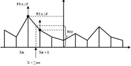
neuronal activation function in ADFUNN
We calculate ∑aw, and find the two
neighbouring f-points that bound ∑aw. Two proximal f-points are adapted separately, on a proportional basis. The proximal-proportional value P1 is (Xn+1 - x)/(Xn+1 – Xn) and value P2 is (x - Xn)/(Xn+1 - Xn). Thus, the change to each point will be in proportion to its proximity to x. We obtain the output error and adapt the two proximal f-points separately, using a function modifying version of the delta rule, as outlined in following to calculate ∆f.
The following is a general learning rule for ADFUNN:
The weights and activation functions are adapted in parallel, using the following algorithm:
A = input node activation, E = output node error.
WL, FL: learning rates for weights and functions.
Step1: calculate output error, E, for input, A. Step2: adapt weights to each output neuron:
∆w = WL • Fslope • A • E w' = w + ∆w
weights normalisation
Step3: adapt function for each output neuron: ∆f (∑aw) = FL • E
f'1 = f1 + ∆f • P1, f'2 = f2 + ∆f • P2
Step4: f (∑aw) = f' (∑aw); w = w'.
Step5: randomly select a pattern to train Step6: repeat step 1 to step 5 until the output error tends to a steady state.
8. Snap-drift ADaptive FUnction
Neural Network (SADFUNN) on
Optical and Pen-Based Recognition of
Handwritten Digits
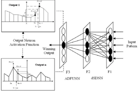
SADFUNN is shown in Figure 8. Input patterns are introduced at the input layer F1, the distributed SDNN (dSDNN) learns to group them. The winning F2 nodes, whose prototypes
[image:11.595.311.544.197.350.2]best match the current input pattern, are used as the input data to ADFUNN. For each output class neuron in F3, there is a linear piecewise function. Functions and weights and are adapted in parallel. We obtain the output error and adapt the two nearest f-points, using a function modifying version of the delta rule on a proximal-proportional basis.
Figure 8: Architecture of the SADFUNN
network
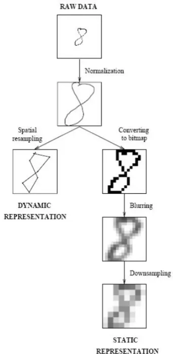
8.1. Optical and Pen-Based Recognition of Handwritten Digits Datasets
These two complex cursive-letter datasets are those of handwritten digits presented by Alpaydin et. al [16, 17]. They are two different representations of the same handwritten digits. 250 samples per person are collected from 44 people who filled in forms which were then randomly divided into two sets: 30 forms for training and 14 forms by distinct writers for writer-independent test.
The optical one was generated by using the set of programs available from NIST [18] to extract normalized bitmaps of handwritten digits from a pre-printed form. Its representation is a static image of the pen tip movement that have occurred as in a normal scanned image. It is an 8 x 8 matrix of elements in the range of 0 to 16 which gives 64 dimensions. There are 3823 training patterns and 1797 writer-independent testing patterns in this dataset.
display and a cordless stylus. The raw data consists of integer values between 0 and 500 at the tablet input box resolution, and they are normalised to the range 0 to 100. This dataset’s representation has eight(x, y) coordinates and thus 16 dimensions are needed. There are 7494 training patterns and 3498 writer-independent testing patterns.
8.2. Snap-drift ADaptive FUnction Neural Network (SADFUNN) on Optical and Pen-Based Recognition of Handwritten Digits
In ADFUNN, weights and activation functions are adapted in parallel using a function modifying version of delta rule. If Snap-Drift and ADFUNN run at the same time, the initial learning in ADFUNN will be redundant. It can only optimise once Snap-Drift has converged; and therefore ADFUNN learning starts when Snap-drift learning has finished.
[image:12.595.331.502.71.420.2]All the inputs are scaled from the range of {0, 16} to {0, 1} for the optical dataset and from {0, 100} to {0, 1} for best learning results. Training patterns are passed to the Snap-Drift network for feature extraction. After a couple of epochs (feature extraction learned very fast in this case, although 7494 patterns need to be classify, but every 250 samples are from the same writer, many similar samples exist), the learned dSDNN is ready to supply ADFUNN for pattern recognition. The training patterns are introduced to dSDNN again but without learning. The winning F2 nodes, whose prototypes best match the current input pattern, are used as the input data to ADFUNN.
Figure 9: The processing of converting the
dynamic (pen-based) and static (optical) representations
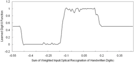
Figure 10: Digit 1 learned function in optical
[image:13.595.311.528.70.167.2]dataset using SADFUNN
Figure 11: Digit 1 learned function in pen-based
dataset using SADFUNN
Now the network is ready to learn using the general learning rule of ADFUNN outlined in section 2. By varying the number of snap-drift neurons (features) and winning features number in F2, within 200 epochs in each run, about 99.53% and 99.2% correct classifications for the best can be achieved for the training data for the optical and pen-based datasets respectively. We get the following output neuron functions (only a few learned functions listed here due to space limitation):
Figure 12: Digit 8 learned function in optical
[image:13.595.51.268.226.329.2]dataset using SADFUNN
Figure 13: Digit 8 learned function in pen-based
dataset using SADFUNN
9. Results
We test our network using the two writer-independent testing data for both of the optical recognition and pen-based recognition tasks. Performance varies with a small number of parameters, including learning rates FL, WL, the number of snap-drift neurons (features) and the number of winning features.
Figure 14: The performance of training and testing
for optical dataset using SADFUNN
Figure 15: The performance of training and testing
for pen-based dataset using SADFUNN
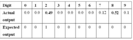
[image:13.595.311.542.359.477.2] [image:13.595.311.541.516.632.2] [image:13.595.52.271.545.647.2]The following are examples of some misclassified patterns from SADFUNN for optical recognition case.
Figure 16: Digit 9 misclassified to digit 5
As we can see above a digit 9 pattern was misclassified to digit 5 which has the largest output. The upper part of digit 5 is almost looped, making the 5 similar to a 9.
[image:14.595.52.268.324.390.2]Figures 17 and 18 illustrate similar confusions
[image:14.595.51.267.425.493.2]Figure 17: Digit 2 misclassified to digit 8
Figure 18: Digit 3 misclassified to digit 9
10. Related Work on the same data
Using multistage classifiers involving a combination of a rule-learner MLP with an exception-learner k-NN [19], the authors of the two datasets reported 94.25% and 95.26% accuracy on the writer-independent testing data for optical recognition and pen-based recognition datasets respectively [16, 17]. Patterns are passed to a MLP with 20 hiddens, and all the rejected patterns are passed to a k-nearest neighbours with k = 9 for a second phase of learning.
For the optical recognition task, 23% of the writer-independent test data are not classified by the MLP. They will be passed to k-NN to
give a second classification. In our single network combination of a single layer Snap-Drift and a single layer ADFUNN (SADFUNN) network only 5.01% patterns were not classified on the testing data. SADFUNN proves to be a highly effective network with fast feature extraction and pattern recognition ability. Similarly, with the pen-based recognition task, 30% of the writer-independent test data are rejected by the MLP, whereas only 5.4% of these patterns were misclassified by SADFUNN.
and achieves similar results. It will be a straight forward process to apply it to many other domains.
A feed forward neural network trained by Quickprop algorithm, which is a variation of error back propagation is used for on-line recognition of handwritten alphanumeric characters by Chakraborty [21]. Some distorted samples in numerals 0 to 9 are used which are different from the dataset used in this paper. Good generalization capability of the extracted feature set is reported.
11. Conclusions
In this paper, following on from recent work in our research programme on modal forms of neural network learning [3], [22], [23], [24] we explored unsupervised Snap-Drift and its combination with a supervised ADFUNN, to perform classification. In addition to performing effective unsupervised analysis, based on groupings of patterns that share both holistic and specific similarities, Snap-Drift also proves very effective and rapid in extracting distinct features from the complex datasets such as the cursive-letter datasets. Experiments show only a couple of epochs are enough for the feature classification. It helps the supervised single layer ADFUNN to solve these linearly inseparable problems rapidly without any hidden neuron. In combination within one network (SADFUNN), these two methods, each of which contain two modes of learning, together exhibited higher generalisation abilities than MLPs, despite being much more computationally efficient, since there is no propagation of errors. In SADFUNN it is also easier to optimise the number of hidden nodes since performance increases when nodes are added and then levels off, whereas with back-propagation methods it tends to increase then decrease.
Acknowledgements
Part of this work was supported by HEFCE E-Learning Funds. We also acknowledge the input to the project of Mike Kretsis, who wrote the student feedbacks.
References
[1] Lee, S. W., Palmer-Brown, D., Tepper, J., and Roadknight, C. M., Snap-Drift: Real-time, Performance-guided Learning, Proceedings of the International Joint Conference on Neural Networks (IJCNN’2003), 2003, Volume 2, pp. 1412 – 1416.
[2] Lee, S. W., Palmer-Brown, D., and Roadknight, C. M., Performance-guided Neural Network for Rapidly Self-Organising Active
Network Management, Neurocomputing,
Volume 61, pp. 5 – 20.
[3] Donelan, H., Pattinson, Palmer-Brown, D., and Lee, S. W., The Analysis of Network Manager’s Behaviour using a Self-Organising Neural Networks, Proceedings of The 18th European Simulations Multiconference, 2004, pp. 111 – 116.
[4] Lee, S. W., and Palmer-Brown, D., Phrase Recognition using Snap-Drift Learning Algorithm, Proceedings of The International Joint Conference on Neural Networks, 2005, Volume 1, pp. 588-592.
[5] R. Garside, G. Leech and T. Varadi, Manual of Information to Accompany the Lancaster Parsed Corpus: Department of English, University of Oslo, 1987.
[6] Lee, S. W., and Palmer-Brown, D., Phonetic
Feature Discovery in Speech using Snap-Drift, Proceedings of International Conference on Artificial Neural Networks (ICANN'2006), S. Kollias et al. (Eds.): ICANN 2006, Part II, LNCS 4132, pp. 952 – 962.
[7] Brown G., J. Bull and M. Pendlebury,
Assessing Students Learning in Higher Education, Routledge, London, 1997
[8] Higgins E, Tatham L, Exploring the
potential of Multiple Choice Questions in Assessment, Learning & Teaching in Action, Vol 2, Issue 1, 2003
[9] Payne, A., Brinkman, W.-P. and Wilson, F.,
Towards Effective Feedback in e-Learning Packages: The Design of a Package to Support Literature Searching, Referencing and Avoiding Plagiarism, Proceedings of HCI2007 workshop: Design, use and experience of e-learning systems, 2007, pp. 71-75.
International Conference on Advanced Learning Technologies, 5-8 July 2005, pp. 827 – 831. [11] Iahad, N.; Dafoulas, G.A.; Kalaitzakis, E.;
Macaulay, L.A., Evaluation of online
assessment: the role of feedback in learner-centered e-learning, Proceedings of the 37th Annual Hawaii International Conference on System Sciences (HICSS'04) - Track 1 - Volume 1, 2004, pp. 10006.1
[12] Race, P., The Open Learning Feedback, 2nd Ed, London:Kogan Page Ltd, 1994
[13] Scheler G., “Regulation of neuromodulator efficacy: Implications for whole-neuron and synaptic plasticity”, Progress in Neurobiology,
Vol.72, No.6, 2004.
[14] Scheler G., “Memorization in a neural network with adjustable transfer function and conditional gating”, Quantitative Biology,
Vol.1, 2004.
[15] Palmer-Brown D., Kang M., “ADFUNN: An adaptive function neural network”, the 7th International Conference on Adaptive and Natural Computing Algorithms (ICANNGA05), Coimbra, Portugal, 2005.
[16] Alpaydin E., Alimoglu F., for Optical Recognition of Handwritten Digits and Alpaydin E., Kaynak C., for Pen-Based Recognition of Handwritten Digits
http://www.ics.uci.edu/~mlearn/databases/optdi gits/
[17] Alpaydin E., Kaynak C., Alimoglu F., “Cascading Multiple Classifiers and Representations for Optical and Pen-Based Handwritten Digit Recognition”, IWFHR,
Amsterdam, The Netherlands, September 2000. [18] Garris M.D., et al, NIST Form-Based Handprint Recognition System, NISTIR 5469, 1991.
[19] Achtert E., Bohm C., Kroger P., Kunath P., Pryakhin A. and Renz M., "Efficient reverse k-nearest neighbour search in arbitrary metric spaces", Proceedings of the 2006 ACM SIGMOD international conference on Management of data, 2006, Pages 515 – 526. [20] Zhang J., Li Z., “Adaptive Nonlinear Auto-Associative Modeling through Manifold Learning”, PAKDD, 2005, pp.599-604.
[21] Chakraborty B. and Chakraborty G., “A New Feature Extraction Technique for On-line Recognition of Handwritten Alphanumeric
Characters”, Information Sciences, Volume 148, Issues 1-4, December 2002, pp.55-70.
[22] Kang M., Palmer-Brown D., “An Adaptive Function Neural Network (ADFUNN) for Phrase Recognition”, the International Joint Conference on Neural Networks (IJCNN05), Montréal, Canada, 2005.
[23] Lee S. W., Palmer-Brown D., Roadknight C. M., “Performance-guided Neural Network for Rapidly Self-Organising Active Network Management (Invited Paper)”, Journal of Neurocomputing, 61C, 2004, pp. 5 – 20