Modelling of water demand in distribution networks

University of East London Institutional Repository: http://roar.uel.ac.uk

This paper is made available online in accordance with publisher policies. Please scroll down to view the document itself. Please refer to the repository record for this item and our policy information available from the repository home page for further information.

To see the final version of this paper please visit the publisher’s website. Access to the published version may require a subscription.

Author(s):Marriott, Martin John

Article Title:Modelling of water demand in distribution networks Year of publication:2007

Citation:Marriott, M.J., (2007) ‘Modelling of water demand in distribution networks’, Urban Water Journal, 4 (4) 283-286

Link to published version:http://dx.doi.org/10.1080/15730620701464240 DOI:10.1080/15730620701464240

Publisher statement:

This is the author’s version of the work. It is posted here by permission of Taylor

& Francis for personal use, not for redistribution. The definitive version was

published in Urban Water Journal, Volume 4 Issue 4, December 2007, 283-286.

(http://dx.doi.org/10.1080/15730620701464240)

Modelling of water demand in distribution networks

M.J.Marriott

School of Computing and Technology

University of East London

Docklands Campus, University Way, London E16 2RD, UK

Tel: +44 208 223 6261

E-mail: m.j.marriott@uel.ac.uk

Abstract

The allocation of water demand to nodes is compared with uniformly

distributed demand along a pipeline, and it is shown that the nodal

approach produces an upper bound or unsafe solution for pressures in

the distribution network. Although the differences are likely to be minor

for computer models with many nodes, the simplest examples show

differences of up to 25% in head loss between the two approaches.

Terminology and concepts from structural engineering are useful in this

comparison. The results are particularly significant to simplified models

using independently derived values of pipe friction factor.

Keywords: water distribution, Darcy-Weisbach head loss, pipe network

1. Introduction

When water distribution networks are modelled by computer or by

hand calculation, it is usual to group the demand and to apply this at

nodes, rather than to model every individual house connection along

each pipeline. Often to simplify the model, the number of nodes is

kept low, so the pattern of demand in the model can represent a

significant approximation to the real situation. Twort et al. (2000)

outline the benefits of manual analysis using a ‘skeleton layout’ for

preliminary planning. They remind readers that ‘the accuracy of any

computer model is not greater than the accuracy with which nodal

demands can be estimated’. The Haestad publication (Walski et al.

2001) refers to the grouping of water demand at nodes as being a

possible source of error, but which produces relatively minor

differences between computer predictions and actual performance.

The effect of the approximation of allocating demand to nodes is

considered and discussed below, using concepts from structural

engineering which are likely to be part of the general civil engineering

training of many water engineers. These will first be outlined.

2. Structural engineering concepts

A topic studied in structural engineering is the plastic analysis of

frames, with the upper bound (‘unsafe’) and lower bound (‘safe’)

equilibrium, mechanism and yield are necessary and sufficient to

determine the true collapse load factor for a frame. When only two

out of the three conditions are satisfied, the solution may be either an

upper bound or a lower bound to the true solution, as summarised in

Table 1. Clearly an upper bound solution for the collapse load is an

unsafe estimate since this overestimates the true load capacity of the

frame.

Texts such as Williams and Todd (2000) explain that elastic design

methods are based on the safe or lower bound theorem, but that

plastic analysis principally makes use of the unsafe theorem. In the

latter approach, various possible mechanisms are formulated, all

representing upper bounds to the true collapse load, and the

mechanism giving the lowest load factor is deduced to be the critical

case. It may then be checked whether this satisfies all three

conditions and is the true collapse load, or whether in fact the true

collapse mechanism has been overlooked. So there is an awareness

here of whether a calculated result is an upper or lower bound to the

actual solution.

The initial study of structural engineering also involves considering

the effects of point loads and uniformly distributed loads on beams.

Plenty of examples are contained in introductory texts such as Smith

(2001). Clearly the representation of loads in this way involves the

3. Application to hydraulic modelling

The concept of uniformly distributed loads, and of upper bound

solutions, that are familiar in structural engineering, may prove to be

useful ideas when considering a water distribution network. Demand

may be considered as uniformly distributed along pipelines, for

comparison with results obtained from point demands applied at

nodes. The various ways of idealising the system to apply nodal

demands may be compared, and it will be shown that these represent

upper bound or unsafe estimates in relation to the true solution.

Consider a pipeline AB as part of a network. The demand may be

taken to be uniformly distributed between A and B, along the length L

of the pipeline. In an urban situation this would closely represent the

reality of many house connections along the length of a distribution

main.

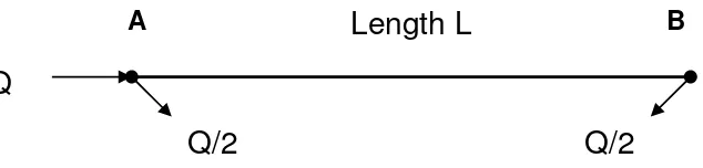
For simplicity, consider that the flow at node B is zero, and the

incoming flow rate at A is equal to Q, as shown in Fig.1. The

uniformly distributed demand is therefore Q/L where L is the length of

the pipeline AB. Frictional head losses will be evaluated using the

Darcy-Weisbach friction formula, in the form

2 5

2 2 2

f KQ

D g

LQ 8 gD 2

LV

h =

π λ = λ

= (1)

where g (m/s2) is the acceleration due to gravity, D (m) is the internal

pipe diameter, L (m) is the length of pipeline with flow at a mean

pipeline resistance, all with S.I. units as shown in brackets. The

dimensionless pipe friction factor λ will be considered to be constant

with flow rate, as in the rough turbulent region, but results may also be

derived using alternative formulae such as Hazen-Williams for the

transitional turbulent region.

For the situation in Fig. 1, with a flow rate varying linearly from Q at

node A down to zero at node B, the total head loss hfAB between A

and B is evaluated as follows:

(

)

fAB

∫

     − π λ

= (2)

yielding 3 KQ D g 3 LQ 8 h 2 5 2 2 fAB = π λ = (3)

This value hfAB in equation (3) will be taken to represent the true value.

Consider now the demand grouped at nodes A and B, as shown in

Fig. 2. The head loss hf1 may be calculated for this idealisation as

follows: 4 KQ D g LQ 2 2 Q D g L 8 h 2 5 2 2 2 5 2 1 f = π λ =       π λ

= (4)

So treating the pipeline AB as one length with the demand allocated

equally to the end nodes, it is found by comparing equations (3) and

(4) that the calculated head loss hf1 is related to the true value by

fAB 1

f h

4 3

h = , and that the head loss is therefore underestimated by

If the pipeline AB is divided into two lengths, as shown in Fig.3,

with the demand divided in two, and then split between the nodes as

shown, the calculated head loss hf2 is as follows:

_fAB 5 2 2 2 2 5 2 2 f h 16 15 D g 2 LQ 5 4 Q 4 Q 3 2 L D g 8 h = π λ =               +             π λ

= (5)

So in this case the head loss is underestimated by one sixteenth of

the true value.

A general expression may be deduced for such a pipeline split in

this way into n lengths, that the head loss hfn is an underestimate by

1/(2n)2 of the head loss that results from uniformly distributed demand.

4. Loop example

Similar analysis may be applied to loops that form parts of pipe

networks. A simple symmetrical example shown in Fig.4 comprises a

square WXYZ with sides of pipework length L and resistance K. With

demand allocated equally to the four nodes W, X, Y and Z as shown,

the head loss from the supply point at node W to the farthest node Y

is given by:

64 KQ 10 8 Q K 8 Q 3 K h 2 2 2

f  =

     +       = (6)

This example may be seen to be similar to the pipeline of Figure 3. If

the demand is considered to be uniformly distributed around the

square, the resulting head loss obtained may be deduced from

(

)

6 KQ 3

2 Q K 2 h

2 2

fWY = = (7)

Comparison of equations (6) and (7) shows that the nodal approach in

(6) underestimates the head loss by one sixteenth, when compared

with the uniformly distributed result.

5. Discussion of implications

Usually the objective of calculating head losses, is to ensure that

at least a certain minimum acceptable pressure is provided to

consumers, as one of the level of service criteria. Therefore it may be

seen that the underestimation of head loss resulting from the various

approximations allocating demand to nodes, will result in

overestimates or upper bound solutions for the available pressure

heads.

Dividing the network into a greater number of pipe lengths and

nodes will reduce the inaccuracy, which is seen above to be inversely

related to the square of the number of lengths into which the pipeline

is divided.

The maximum error shown in the above calculations amounts to

one quarter or 25% of the head loss for uniformly distributed demand.

Such possible errors should be noticed when a very simplified model

is used, perhaps to provide an overview of a complex situation.

The above comments apply particularly where the pipe friction

friction values in the model have been obtained by calibrating the

model against measured values of flow and pressure, then the above

effect will have been accounted for in the deduced friction values.

6. Conclusions

Concepts of uniformly distributed loads and upper bound solutions

from structural engineering have been used in pipe network analysis

to compare head losses resulting from various idealised situations.

It has been demonstrated that idealisations of pipe networks that

place the demand at nodes are in effect upper bound or ‘unsafe’

solutions when used to estimate the minimum pressures available to

consumers.

The maximum error demonstrated in head loss for a single pipe is

an underestimate by 25%, compared with uniformly distributed

demand.

Possible errors of this type arise when running very simplified

models, and will be reduced by increasing the number of nodes in the

model.

It is noted that the above comments apply where pipe friction

factors have been independently derived, and not adjusted as part of

References

Heyman, J. (1974) Beams and framed structures (2nd ed.). Pergamon,

Oxford.

Smith, P.S. (2001) Introduction to structural mechanics. Palgrave,

Basingstoke.

Twort, A.C., Ratnayaka, D.D. and Brandt, M.J. (2000) Water supply (5th

ed.). Arnold, London, reprinted by Butterworth-Heinemann, Oxford, 2001.

Walski, T.M., Chase, D.V. and Savic, D.A. (2001) Water distribution

modeling, Haestad press, Waterbury, CT.

Williams, M.S. and Todd, J.D. (2000) Structures: theory and analysis.

Macmillan, Basingstoke.

Table 1. Structural design of frames by plastic analysis

Condition Upper bound theorem

(unsafe)

Lower bound theorem (safe)

Equilibrium Satisfied Satisfied

Mechanism Satisfied Not satisfied

Fig. 1. Uniformly distributed demand along pipeline

Fig. 2. Demand grouped at nodes with pipeline as one length

Fig. 3. Demand grouped at nodes with pipeline divided into two equal lengths

Q

A B

Uniformly distributed demand Q/L

Length L

Q

A

_{Length L}

Q/2

Q/2

Q

A

_L/2

Q/4

Q/4

Q/4

L/2

Q/4

Q/4

Q/4

Fig. 4. Simple loop example with demand allocated equally to nodes

Q/4

Q/4

Q/4

Q/4

Q/4

Q/4

Q/4

Q/4

Y Z

Q

L

e

n

g

th

L