A Hybrid Multiobjective RBF-PSO Method for Mitigating DoS Attacks in
Named Data Networking
Amin Karami∗, Manel Guerrero-Zapata
Computer Architecture Department (DAC), Universitat Polit`ecnica de Catalunya (UPC), Campus Nord, C. Jordi Girona 1-3. 08034 Barcelona, Spain
Abstract
Named Data Networking (NDN) is a promising network architecture being considered as a possible replacement for the current IP-based (host-centric) Internet infrastructure. NDN can overcome the fundamental limitations of the cur-rent Internet, in particular, Denial-of-Service (DoS) attacks. However, NDN can be subject to new type of DoS attacks namely Interest flooding attacks and content poisoning. These types of attacks exploit key architectural features of NDN. This paper presents a new intelligent hybrid algorithm for proactive detection of DoS attacks and adaptive mit-igation reaction in NDN. In the detection phase, a combination of multiobjective evolutionary optimization algorithm with PSO in the context of the RBF neural network has been applied in order to improve the accuracy of DoS attack prediction. Performance of the proposed hybrid approach is also evaluated successfully by some benchmark problems. In the adaptive reaction phase, we introduced a framework for mitigating DoS attacks based on the misbehaving type of network nodes. The evaluation through simulations shows that the proposed intelligent hybrid algorithm (proactive detection and adaptive reaction) can quickly and effectively respond and mitigate DoS attacks in adverse conditions in terms of the applied performance criteria.
Keywords: Named Data Networking, DoS attacks, Intelligent Hybrid Algorithm, RBF neural networks, Particle Swarm Optimization, NSGA II
1. Introduction
In recent years there have been several efforts to de-sign new network architectures for a viable and vital replacement for the current IP-based Internet [1, 2, 3]. These new architectures are designed to better cope with the fundamental limitations of the Internet in supporting today’s content-oriented services [4, 5]. In particular, there have been significant efforts regarding security, privacy, better mobility, scalability and efficient content distribution [6, 7]. Strong security has been one of the main design requirements for these architectures [8, 9]. Named Data Networking (NDN) [10] is one of these architectures as an ongoing research effort that aims to move the Internet into the future with a content-centric approach. NDN is a prominent example of
∗Corresponding author, Telephone: 0034-934011638
Email addresses:[email protected](Amin Karami),
[email protected](Manel Guerrero-Zapata) URL:http://personals.ac.upc.edu/amin(Amin Karami),http://personals.ac.upc.edu/guerrero(Manel Guerrero-Zapata)
Content-Centric Networking (CCN, also referred to as Information-Centric Networking (ICN) or Data-Centric Networking (DCN)) design. In CCN, content -rather than hosts, like in IP-based design- plays the central role in the communications [11, 12].
The first goal of any protection scheme against DoS at-tack is the early detection (ideally long before the de-structive traffic build-up) of its existence [22, 21]. In or-der to disarm DoS/DDoS attacks and any deviation, not only the detection of the malevolent behavior must be achieved, but the network traffic belonging to the attack-ers should be also blocked [23, 24, 25]. Thus, a predic-tor (detecpredic-tor) should take an appropriate action to thwart the attacks and should be able to adjust itself to the changing dynamics of the anomalies/attacks [20, 26]. In an attempt to tackle with the new kinds of DoS attacks and the threat of future unknown attacks and anoma-lies, many researchers have been developing intelligent learning techniques as a significant part of the current research on DoS attacks detection [16, 27]. The most popular approach for DOS/DDoS attacks prediction is using Artificial Neural Networks (ANNs) classification [28, 29, 30]. ANNs have become one of the most vi-tal and valuable tools in solving many complex prac-tical problems [31, 32], among which the Radial basis function (RBF) neural networks have been successfully applied for solving dynamic system problems, because they can predict the behavior directly from input/output data [33, 34, 35]. RBF networks have many remarkable characteristics, such as simple network structure, strong learning capacity, better approximation capacities and fast learning speed. The difficulty of applying the RBF networks is in network training which should select and estimate properly the input parameters including cen-ters and widths of the basis functions and the neuron connection weights [32, 36, 37]. In order to find the most appropriate parameters, an optimization algorithm can be used [38, 39]. An optimization algorithm will attempt to find an optimal choice that satisfies defined constraints and make an optimization criterion (perfor-mance or cost index) maximize or minimize [38, 40]. Hence, to improve the prediction accuracy and robust-ness of the RBF network, network parameters (centers, widths and weights) should be simultaneously tuned [32]. Some of the existing algorithms to achieve that are given in [32, 36, 41, 42, 43]. Almost all algorithms com-pute the optimal estimation of the basis function centers by mean of error minimization, i.e., accuracy based on Mean-Square Error (MSE) [36, 43, 44, 45]. However, MSE is not suitable for determining the optimal position of basis function centers. Since the MSE decreases, the number of centers increases [46]. To accomplish this task, we develop our proactive detection algorithm for globally well-separating units’ centers and their local optimization by MSE (decreasing the error caused by corresponding data points and their centers, separately). But the optimal placement and well-separated centers
can increase MSE [47]. It is generally accepted that well-separated (external separation of) centers and their local optimization (internal homogeneity) are conflict-ing objectives [46, 48]. This trade-offis a well-known problem as the Multiobjective Optimization Problem (MOP) [49, 50, 51, 52]. This paper applies NSGA II (Non-dominated Sorting Genetic Algorithm) proposed by Deb et al. (2002) to solve this problem, as it has recently been frequently applied to various scenarios [53, 54, 55, 56]. On the other hand, for (near) optimal estimation and adjustment of two others RBF parame-ters (units’ widths and output weights), we implement Particle Swarm Optimization (PSO) that favors global and local search of its interacting particles which has proved to be effective in finding the optimum in a search space [57, 58, 59].
When the DoS attacks by the proposed intelligent pre-dictor are identified, the second phase (i.e., adaptive mitigation reaction) is triggered by enforcing explicit limitations against adversaries. The contribution of this paper is summarized in three objectives. The first ob-jective of this paper is to develop an algorithm to re-solve the hybrid learning problem of a RBF network us-ing multiobjective optimization and particle swarm op-timization to obtain a simple and more accurate RBF network-based classifier (predictor). The second objec-tive is utilization of this optimized RBF network-based predictor in proactive detection of the DoS/DDoS at-tacks in NDN. The third objective is introducing a new algorithm to enable NDN routers to perform quickly and effectively adaptive reaction (recovery) from net-work problems, in order to keep track of legitimate data delivery performance and effectively shutting down ma-licious users’ traffic.
in detail. Section 8 describes the proposed hybrid intel-ligent method. Section 9 examines the detection (clas-sification) phase of the proposed hybrid algorithm on several benchmark problems. Evaluation environment is described in Section 10 in detail. Section 11 pro-poses our countermeasure including proactive detection and adaptive reaction mechanism against DoS attacks in NDN. Detailed analysis and discussions are explained in Section 12. Finally, Section 13 draws conclusions.
2. NDN overview
NDN is a novel next-generation Internet archi-tecture based on the principle of CCN (Content-Centric Networking) paradigm, where contents are re-trieved by their names instead of by the network ad-dresses where they are hosted [60]. Data names in NDN are hierarchically structured, e.g., eighth fragment of a youtube video (file) would be named
/youtube/videos/A7m5I6n8kVUw/8. NDN is one
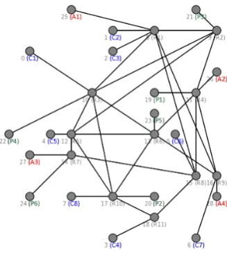
of the five NSF-sponsored Future Internet Architecture (FIA) [21]. It supports two types of messages:Interest
[image:3.595.82.269.395.472.2]andcontent (Fig. 1). A consumer asks for a content
Figure 1: CCN packet types [12]
by routing an Interest request using name prefixes in-stead of today’s IP prefixes. Interest packet is routed towards the location of the origin content where it has been published. Any router and middle node on the way checks its cache for matching copies of the requested content. If a cached copy of any piece of Interest request is found, it is returned to the requester along the path the request came from. On the way back, all the middle nodes store a copy of content in their caches to answer to probable same Interest requests from subsequent re-quests [16]. Each NDN router maintains three major data structures includingForwarding Information Base
(FIB),Pending Interest Table(PIT) andContent Store
(CS) or buffer memory. FIB is a lookup table used to determine interfaces for forwarding incoming Interests packets which contains [name prefix, interface num-ber] entries. Another lookup table is PIT which con-tains outstanding entries [Interest prefix,arrival inter-face]. When a NDN router receives an Interest packet,
it first checks its CS (cache). If there is no copy of the requested content, it looks up its PIT table. If the same name is already in the PIT and the arrival interface of the present Interest is already in the set ofarrival interface
of the corresponding PIT entry, the Interest is discarded. If a PIT entry for the same name exists, the router up-dates the PIT entry by adding a new arrival interface to the set. The Interest is not forwarded further. Other-wise, the router creates a new PIT entry and forwards the present Interest using its FIB [12, 61].
3. DoS attacks in NDN
The new variations of DoS attacks might be quite ef-fective against NDN. An adversary can take advantage of two features unique in NDN routers as CS and PIT to mount DoS/DDoS attacks into NDN. There are two major categories of DoS attacks in NDN infrastructure [20, 62]:
1. Interest Flooding Attack (IFA): It is partly due to the lack of authentication of Interest packets (source). Anyone can generate Interests packets and any middle router (node) only knows that a particular Interest packet entered on a specific in-terface.
2. Content/Cache Poisoning: The adversary tries to make routers forward and cache corrupted or fake data packets in order to prevent consumers from retrieving the original (legitimate) content.
3.1. Interest Flooding Attack
In this type of attack, the adversary (controlling a set of possibly geographically distributed zombies) gener-ates a large number of Interest packets aiming to (1) overwhelm PIT table in routers in order to prevent le-gitimate users to satisfied their Interest packets and (2) swamp the target content producers [20]. There are three types of Interest flooding attacks, based on the type of content requested [20]:
1. existing or static: it is quiet limited since in-network content caching provides a built-in coun-termeasure. If several zombies from different paths generate large number of Interest packets for an existing content which settles in all intervening routes’ caches, these Interest packets for the same content can not propagate to the producer(s) since they are satisfied by cached copies.
producer(s), thus consuming bandwidth and router PIT table. Also, content producer might waste con-siderable computational resources due to the sign-ing the content (per-packet operation) which is it-self expensive.
3. non-existent (unsatisfied Interests): Such Interest packets cannot be collapsed by routers, and are routed toward the content producer(s). This type of Interest packets take up space in router PIT table until they expire. A large number of non-existent Interest packets in PIT table lead to legitimate In-terest packets being dropped in the network.
4. Related work
As a new Internet architecture proposal, there is very limited work recently regarding to mitigation of DoS/DDoS attacks in Named Data Networking. Gasti et al. [20] performed initial analysis of NDN’s resilience to DoS attacks. This work identifies two new types of attacks specific to NDN (Interest flooding and con-tent/cache poisoning) and discusses effects and poten-tial countermeasures. However, the paper does not ana-lyze DoS attacks and their countermeasures. Afanasyev et al. [15] presented three mitigation algorithms (token bucket with per interface fairness, satisfaction-based In-terest acceptance and satisfaction-based pushback) that allow routers to exploit their state information to thwart Interest flooding attacks. Among these three miti-gation algorithms, satisfaction-based pushback mecha-nism could effectively shut down malicious users while preventing legitimate users from service degradation. This work uses a simple and static attackers model (sending junk Interests as fast as possible), and it does not consider intermediate router’s cache and always for-wards all the way to the producer. Compagno et al. [21] introduced a framework for local and distributed Inter-est flooding attack mitigation, in particular, rapid gener-ation of large numbers of Interest for non-existent con-tents that saturate the victim router’s PIT. Authors sim-ulated a simple attackers model, and their countermea-sure has been able to use around 80-90% of the available bandwidth in the most cases during the attacks. Dai et al. [63] proposed Interest traceback as a counter mea-sure against NDN DDoS attacks, which traces back to the originator of the attacking Interest packets. In this paper, when PIT exceeds its threshold, Interest trace-back is triggered. This method responds to the attack by generating spoofed Data packets to satisfy the long-unsatisfied Interest packets in the PIT by tracing back to the Interest originators. This method is not proac-tive, makes overhead in the network by increasing of
made spoofed contents. It leads to middle routers cache bogus contents. This paper also assumes that the long-unsatisfied Interests in the PIT is adversary and others unsatisfied Interest are normal usages. Another short-coming of this method is that the router drops the in-coming packet rate of the interface which has too many long-unsatisfied Interest packets. As a result of this in-dependent decision, the probability of legitimate Inter-ests being forwarded decreases rapidly as the number of hops between the content requester and producer. Choi et al. [18] provided an overview of threats of Inter-est flooding attacks for non-existent contents on NDN. Authors simulated and explained the effect of Interest flooding DoS attacks by a simple scenario over the qual-ity of services for legitimate Interest packets from nor-mal users due to PIT full. However, they do not analyze DoS attacks and their countermeasures.
5. RBF neural networks
Radial Basis Function (RBF) is a kind of feed-forward neural networks, which were developed by Broomhead and Lowe in 1998 [64]. This type of neu-ral networks use a supervised algorithm and have been broadly employed for classification and interpolation re-gression [65]. As compared to other neural networks, RBF neural networks have better approximation charac-teristics, faster training procedures and simple network architecture. For these reasons, researchers have con-tinued working on improving the performance of RBF learning algorithms [66, 67]. The RBF neural networks have three layers architecture including a single hidden layer of units. The first layer has ninput units which connects the input space to the hidden layer. The hid-den layer hasmRBF units, which transforms the input units to the output layer. The output layer, consisting of
llinear units. The output layer implements a weighted sum of hidden unit outputs. The input layer is non-linear while the output is linear. Due to non-linear approxima-tion properties in RBF, this type of networks are able to model the complex mappings [34, 37]. The real output in output layer is given by:
ys(X)=
k
X
j=1 wjsφ(
P−Cj
σj
) f or 1≤s≤l (1)
Whereys iss-th network output,Pis an input pattern, wjsis the weight of the link betweenj-th hidden neuron
ands-th output neuron,Cjis the center of thej-th RBF
unit in the hidden layer, and σj is the width of thej
(activation) function. The Gaussian activation function is used in this paper, which is given by [68]:
φj(r)=exp(−
P−Cj
2
2σ2 j
) j=1,2,3, ...,p (2)
[image:5.595.65.296.205.325.2]Whereris the variable of radial basis function (φ).
Figure 2: Schematic of the NSGA II procedure
6. Particle Swarm Optimization (PSO)
PSO was initially introduced in 1995 by James Kennedy and Russell Eberhart as a global optimization technique [69]. It was inspired by the social behavior of a bird flock or fish school. It is a population based meta-heuristic method that optimizes a problem by ini-tializing a flock of birds randomly over the search space where each bird is referred as aparticle and the popu-lation of particles is calledswarm[70]. Each particle is a candidate solution to the problem which is assigned a velocity vector and has a memory which helps it in remembering its previous best position (known as lo-cal best, lbest). The particles move iteratively around in the search space according to a simple mathemati-cal formula over the particle’s position and velocity to find the global best position (known asGbest). In the
n-dimensional search space, the position and the veloc-ity ofi-th particle at t-th iteration of algorithm is de-noted by vectorXi(t)=(xi1(t),xi2(t), ...,xin(t)) and vec-torVi(t)=(vi1(t),vi2(t), ...,vin(t)), respectively. Usually a fitness function is the objective function to be min-imized or maxmin-imized. Hereafter, a record of the best position of particle based on the fitness function value is kept in process. The best previously visited position of the particle i at current stage is denoted by vector
lbesti=(lbesti1,lbesti2, ...,lbestin) as the personal best.
The position of the best objective function value until the current stage is also recorded as the global best po-sition denoted byGbest = (gbest1,gbest2, ...,gbestn).
The velocity and position of particle iat iterationk+1 can be calculated according the following equations:
Vi(k+1)=ωVi(k)+c1r1(lbesti(k)−Xi(k)) +c2r2(gbest(k)−Xi(k)) (3)
Xi(k+1)=Xi(k)+Vi(k+1) (4)
Whereωis the inertia weight,c1 (cognitive parameter) and c2 (social parameter) are constants which control the search space between the local best position and the global best position (generallyc1 =c2 =2 [48]). Pa-rameters r1 andr2 are random numbers uniformly dis-tributed within [0 1]. Since larger ω performs more efficient global search and smaller one performs more effective local search, Eberhart and Shi [71] used Eq. (5) that properly balances between exploration (global search) and exploitation (local search) to avoid prema-ture convergence to a local optimum.
ω=ωmax−t·
(ωmax−ωmin)
T (5)
Whereωmax, ωmin,T andtdenote the maximum inertia
weight, the minimum inertia weight, the total and the current number of iterations, respectively.
7. Non-dominated Sorting Genetic Algorithm (NSGA) II
NSGA II is one of the most widely and popular multi-objective optimization algorithms with three consider-able properties including fast non-dominated sorting ap-proach, fast crowded distance estimation procedure and simple crowded comparison operator [72]. Fig. 2 shows the NSGA II procedure. Generally, NSGA II can be roughly detailed as following steps [72, 73, 74]:
Step 1: Population initialization
A set of random solutions (chromosomes) with a uni-form distribution based on the problem range and con-straint are generated. The first generation is a N×D
matrix. N andDare identified as the number of chro-mosomes and decision variables (genes), respectively.
Step 2: Non-dominated sort
Sorting process based on non domination criteria of the initialized population.
Step 3: Crowding distance
Chromosomes are classified to the Pareto fronts using:
dIj =
M
X
m=1 fI
m j+1
m −f Im
j−1
m fMax
m −fmMin
(6)
Where, dIj is crowded distance of jth solution, M is
number of objectives, fI
m j+1
m and f Im
j−1
Figure 3: The overview of the proposed DoS mitigation method in NDN
objective for (j−1)th and (j+1)th solution, fMax m is
maximum value ofmth objective function among solu-tions of the current population, fMin
m is minimum value
of mth objective function among solutions of the cur-rent population, Ij is the jth solution in the sorted list and (j−1) and (j+1) are two nearest neighboring so-lutions on both sides of Ij. Afterwards, the algorithm searches the nearest points (solutions) with more value of dIj. Solutions in the best-known Pareto set should be uniformly distributed and diverse over of the Pareto front in order to provide the decision maker a true pic-ture of trade-offs. Then, Pareto fronts are ranked from the best to the worst.
Step 4: Selection
The selection of chromosomes is carried out to select appropriate chromosomes (parents) using the crowded tournament operator. The crowded tournament opera-tor compares different solutions with two criteria, (1) a non-dominated rank and (2) a crowding distance in the population. In this process, if a solution dominates the others, it will be selected as the parent. Otherwise, the solution with the higher value of crowding distance (highest diversity) will be selected.
Step 5: Genetic algorithm operators
There are a variety of recombination (crossover) and mutation operators.
Step 6: Recombination and selection
The offspring population is combined with the current generation population and the total population is sorted based on non-domination. The new generation is filled by chromosomes from each front subsequently until the population size exceeds the current population sizeN.
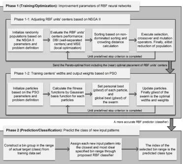
8. The proposed hybrid intelligent method for DoS mitigation in NDN
In this section, we introduce our method, a two-phase framework for mitigating DoS attacks in NDN. The first phase being proactive detection (see section 8.1) and the
second one adaptive reaction (see section 11.2). The proposed predictor in the first phase is a global frame-work so that we can use the predictor in other netframe-works. In this paper, we apply the proposed predictor success-fully on some benchmark problems and NDN and leave further investigations in other networks to future work. A diagram of the two phases of the proposed method is shown in Fig. 3.
8.1. The proposed intelligent classifier (predictor)
This section presents the details of proposed intel-ligent algorithm for classification problems. Our ap-proach composes of two main phases. It is depicted in Fig. 4. Each phase is given in the next subsections.
8.1.1. Phase 1: Improvement of RBF parameters
In the first phase -training (optimization)- we intro-duce a new hybrid optimization approach for designing RBF neural networks which can be implemented for real-world problems. Firstly, a new multiobjective optimization algorithm as NSGA II for adjusting centers of the RBF units is introduced. This algorithm obtains various non-dominated sets that provide an appropriate balance between two conflicting objectives: well-separated and local optimization of RBF centers. Secondly, PSO algorithm has been applied to simul-taneously tune widths of the RBF units and output weights through well-placed centers. The algorithm is presented below:
A. First part(adjustingRBFunits’centers based on NSGA II):
1. Problem definition:
1-1- population size (N), maximum iteration (IterMax), crossover percentage (pCrossover),
number of parents (offspring) after crossover op-erator (nCrossover = 2 ×round(pCrossover ×
N
2)), mutation percentage (pMutation),
Figure 4: Proposed intelligent algorithm for more accurate classification
round(pMutation×N)), mutation rate (mu), mu-tation step size (sigma=0.1).
2. Initialize population:
2-1- Generate the initial populations (individuals)
P, includingP1,P2, ...,PN.
2-2- Calculate the two conflicting cost functions as DBI and MSE (presented in section 8.1.3) for each population.
2-3- Rank all populations according to their non-dominance.
2-4- Calculate the crowding distances for all popu-lations to keep the population diversity (Eq. 6). 2-5- Sort the non-dominated solutions in descend-ing crowddescend-ing distance and rank values.
3. NSGA II main loop:
3-1- Execute the evolution process including crossover and mutation operators:
a. Execute crossover operator, PopCrossover
(this paper adopts the two-point crossover). b. Execute mutation operator, PopMutation (A
Gaussian distributed random number with mean zero and variance 1 is used [75, 76]).
c. Merge populations:
P=[P PopCrossover PopMutation].
3-2- Run steps 2-3 (rank), 2-4 (crowding distance) and 2-5 (sort) over the mergedP.
3-3- Truncate/Select the generated populationPto the range of population size:P=P(1 :N). 3-4- Run steps 2-3 (rank), 2-4 (crowding distance) and 2-5 (sort) over the truncatedP.
3-5- Store Pareto-optimal front (non-dominated set) in the archive asPF1.
3-6- Repeat Step 3 until termination condition (IterMax) is reached.
3-7- Keep the finalPF1 including the (near) opti-mal placement of RBF units’ centers.
B. Second part(calculating widths of theRBFunits and output weights based onPSOalgorithm):
1-1- population size (N), maximum iteration (IterMax) and number of RBF Kernel obtained fromPF1 in phase A (nKernel).
1-2- Upper and lower bound of width (σ) and weight (w) variables.
1-3- Adjust the PSO parameters: inertia weight (ω) which is linearly decrease by Eq. 5, acceler-ation coefficients (c1 =c2 =2), and two random numbers (r1 andr2) which distributed uniformly in [0 1].
2. Initialize population for each particle:
2-1- Generate the initial
popula-tions (particle positions) including
Particle(1),Particle(2), ...,Particle(N):
Particle(i).Position.σ and Particle(i).Position.w.
i=1,2, ...,N.
particle(i).Position.σ = Continuous uniform random numbers betweenσ.Lower andσ.U pper
in size ofnKernel.
particle(i).Position.w = Continuous uniform random numbers betweenw.Lowerandw.U pper
in size ofnKernel.
2-2- Initialize velocity vectors in a feasible space for each particle:
particle(i).Velocity.σ = a nKernal size zero matrix.
particle(i).Velocity.w = a nKernal size zero matrix.
2-3- Evaluate each particle by Gaussian basis function in each RBF units (Eq. 1). Calculate Gaussian basis function with two tuned parameters (σ-centers’ widths- andw-output weights- from PSO) and optimal placement of RBF units’ centers from archivePF1.
2-4- Initially, personal best (lbest) is the current calculated cost.
3. Set the global best (gbest) to a particle with the lowest cost.
4. PSO main loop:
4-1- Update velocity for each particle by Eq. 3. 4-2- Control the lower (Vmin) and upper (Vmax) bounds of velocity:
Vmin ≤ Vit ≤Vmax. Where, i (particle id)=1, 2, ..., N and t (iteration number)=1, 2, ...,IterMax. 4-3- Update position by Eq. 4.
4-4- If the current velocity and position are out-side of the boundaries, they take the upper bound or lower bound. They are multiplied by -1 so that they search in the opposite direction (mirroring to feasible search space).
4-5- Update personal best (lbest): if the current particle cost is better than the previous (recorded
inlbest) particle cost, then set the current particle cost as the personal best.
4-6- Update global best (gbest): if the current per-sonal best is better than the global best, then set the current personal best as the global best in the swarm.
5. Repeat Step 4 until termination condition (MaxIter) is reached. Otherwise,gbestis the optimized RBF units’ widths and output weights.
8.1.2. Phase 2: classification of new input patterns
In the second phase -prediction (classification)- we classify (predict) the class type of new input patterns, which we do not know about their target classes in prior. The classification is calculated by defining bins. Data samples should be normalized into [0 1], when deal-ing with parameters of different units and scales [77]. Since data set is normalized in range of [0 1], bin val-ues should be defined in this range. The number of bin ranges are equal to the number of target classes in train-ing phase. Then, we can determine which data object falls into a specified bin range. For instance, if the num-ber of target class in a particular data set is five classes, then the range of bin values can be organized in the range of [0 0.25 0.5 0.75 1]. Hereafter, constructed RBF neural network from first phase is executed over the input patterns. The RBF output is always a decimal number between [0 1]. This output assigns to the clos-est and most ideal index of specified bin range, e.g., if output=0.65, then the input pattern falls into fourth bin. It means that the predicted class is four. The pseudo-code of classification computation is given below: 1- Define some input parameters:
LowEdge=lower bound of target class.
UpEdge=upper bound of target class.
NumBins=number of target classes in training data set.
BinEdges=Generate linearly spaced vectors between
LowEdgeandU pEdgein the size ofNumBins, where the bin range is equal to the number of target class. 2- Assign input patterns into the closest index of spec-ified bin range. The index of bin range is the predicted classes of input patterns.
Table 1: The four applied benchmark data sets
Data set No. of features No. of classes No. of patterns
Wine 13 3 178
Iris 4 3 150
Ionosphere 34 2 351
8.1.3. Objective functions in NSGA II
Two objective functions are used to evaluate the RBF network units’ centers performance. The two objective functions for minimization problems are:
1. Local optimization based on Mean Square Error (MSE):
Given the set of centers (c), the set of corresponding data objects (x),cxdenotes the center corresponding to thex, andNis the number of data points, MSE can be calculated as:
MS E= 1 N
N
X
i=1
d(xi,cx)2 (7)
2. Well-separated (well-placed) RBF units’ centers based on Davies-Boulding Index (DBI).
Based on our experiments [46], we have found it quite reliable. DBI [78] takes into account both compactness and separation criteria that makes similar data points within the same centers and places other data points in distinct centers. The compactness of a group of data ob-jects with corresponding center is calculated based on the MSE. The separation is measured by the distance between centersciandcj. In general, the DBI is given
by:
1
NC
X
i
maxj,j,i
[n1 i
P
xCid(x,ci)+
1 nj
P
xCjd(x,cj)]
d(ci,cj)
[image:9.595.311.531.132.271.2](8) Where, NC is the number of centers, x is the corre-sponding data objects,niis the number of data objects belonging to the centerci.
Table 2: adjusting RBF units’ centers in Wine
n Pop. Iter. MSE Std. SEM CI (95%) PSO:
20 20 1500 0.19224 0.1235 0.0101 [0.182 0.671] 40 30 2000 0.16474 0.1207 0.0104 [0.176 0.649] 70 35 2500 0.14989 0.1013 0.0088 [0.165 0.572] GA:
20 20 1500 0.19423 0.1242 0.0104 [0.188 0.68] 40 30 2000 0.16532 0.1222 0.0105 [0.196 0.671] 70 35 2500 0.3729 0.1072 0.0093 [0.171 0.583] ICA:
20 20 1500 0.41448 0.1421 0.0123 [0.349 0.907] 40 30 2000 0.3396 0.1235 0.0107 [0.327 0.812] 70 35 2500 0.30012 0.124 0.0107 [0.291 0.777] DE:
20 20 1500 0.38732 0.1484 0.0128 [0.314 0.895] 40 30 2000 0.41173 0.1555 0.0134 [0.318 0.928] 70 35 2500 0.41586 0.1442 0.0125 [0.346 0.911]
9. Benchmarking the proposed intelligent classifier (predictor)
For assurance of robustness and accuracy of our pro-posed intelligent hybrid classifier (predictor), we
ap-Table 3: adjusting RBF units’ centers in Iris
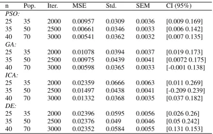
n Pop. Iter. MSE Std. SEM CI (95%) PSO:
25 35 2000 0.00957 0.0309 0.0036 [0.009 0.169] 35 50 2500 0.00661 0.0346 0.0033 [0.006 0.142] 40 70 3000 0.00541 0.0362 0.0032 [0.007 0.135] GA:
25 35 2000 0.01078 0.0394 0.0037 [0.019 0.173] 35 50 2500 0.00975 0.0439 0.0041 [0.0072 0.175] 40 70 3000 0.00598 0.0365 0.0033 [-0.001 0.138] ICA:
25 35 2000 0.02359 0.0666 0.0063 [0.011 0.269] 35 50 2500 0.01497 0.0438 0.0041 [-0.209 0.239] 40 70 3000 0.01332 0.0368 0.0035 [0.037 0.182] DE:
25 35 2000 0.02396 0.0595 0.0056 [0.026 0.26] 35 50 2500 0.02376 0.049 0.0046 [0.05 0.242] 40 70 3000 0.02352 0.0584 0.0055 [0.131 0.153]
Table 4: adjusting RBF units’ centers in Ionosphere
n Pop. Iter. MSE Std. SEM CI (95%) PSO:
40 60 3000 0.90357 0.4709 0.0297 [-0.104 1.763] 50 80 4000 0.81119 0.457 0.0282 [-0.079 1.673] 60 90 4000 0.74164 0.4496 0.0284 [-0.085 1.631] GA:
40 60 3000 1.043 0.4953 0.0299 [-0.111 1.836] 50 80 4000 0.9489 0.4615 0.0285 [-0.086 1.763] 60 90 4000 0.9394 0.4501 0.0278 [-0.093 1.741] ICA:
40 60 3000 2.113 0.5575 0.0344 [0.25 2.436] 50 80 4000 1.9462 0.4792 0.0295 [0.37 2.25] 60 90 4000 1.8535 0.4743 0.0292 [0.347 2.206] DE:
40 60 3000 2.6211 0.5671 0.035 [0.405 2.629] 50 80 4000 2.6249 0.5878 0.0362 [0.358 2.663] 60 90 4000 2.5915 0.5493 0.0339 [0.437 2.59]
Table 5: adjusting RBF units’ centers in Zoo
n Pop. Iter. MSE Std. SEM CI (95%) PSO:
40 50 2000 0.75405 0.23 0.0264 [-0.288 1.289] 50 70 2500 0.67409 0.2622 0.0301 [0.198 1.318] 60 90 3000 0.68884 0.2563 0.0274 [0.249 1.253] GA:
40 50 2000 0.75469 0.2793 0.032 [0.296 1.371] 50 70 2500 0.68008 0.3057 0.0351 [0.201 1.366] 60 90 3000 0.69329 0.2654 0.0281 [0.315 1.277] ICA:
40 50 2000 1.1539 0.303 0.0348 [0.315 1.377] 50 70 2500 0.9867 0.3112 0.0357 [0.334 1.554] 60 90 3000 1.0088 0.2826 0.0324 [0.41 1.518] DE:
40 50 2000 1.96 0.3213 0.0369 [0.733 1.933] 50 70 2500 1.9406 0.2829 0.0325 [0.81 1.919] 60 90 3000 1.8115 0.2736 0.0314 [0.782 1.855]
Table 6: Classification of Wine data set based on RBF-PSO optimization algorithm
n Pop. Iter. Training data set Test data set
MSE Std. CI (95%) SEM Cls. err. MSE Std. CI (95%) SEM Cls. err. Units’ centers by PSO:
20 25 2000 0.00838 0.0912 [-0.157 0.158] 0.00692 2 0.01078 0.109 [-0.208 0.2] 0.01567 2 40 30 2500 0.00586 0.08024 [-0.158 0.157] 0.00676 0 0.01389 0.11475 [-0.25 0.199] 0.01814 3 70 40 3000 0.00519 0.07145 [-0.135 0.146] 0.00617 1 0.01316 0.11656 [-0.22 0.237] 0.0174 3 Units’ centers by GA:
20 25 2000 0.0084 0.093 [-0.164 0.166] 0.00725 1 0.01082 0.10907 [-0.216 0.192] 0.01568 3 40 30 2500 0.00598 0.08227 [-0.171 0.173] 0.00624 1 0.01479 0.11874 [-0.265 0.201] 0.0179 4 70 40 3000 0.00525 0.07254 [-0.137 0.148] 0.00626 2 0.01501 0.12183 [-0.261 0.216] 0.01836 3 Units’ centers by ICA:
20 25 2000 0.00917 0.09615 [-0.188 0.189] 0.0083 1 0.01688 0.13139 [-0.262 0.254] 0.0198 4 40 30 2500 0.00716 0.08496 [-0.166 0.167] 0.00734 1 0.01483 0.11884 [-0.234 0.216] 0.01742 3 70 40 3000 0.00677 0.08255 [-0.159 0.165] 0.00713 1 0.01576 0.12683 [-0.038 0.024] 0.01912 3 Units’ centers by DE:
[image:10.595.71.531.313.460.2]20 25 2000 0.01159 0.10808 [-0.212 0.212] 0.00933 2 0.02135 0.14608 [-0.309 0.264] 0.02202 3 40 30 2500 0.00906 0.09555 [-0.187 0.188] 0.00825 1 0.01401 0.11895 [-0.252 0.211] 0.01778 3 70 40 3000 0.00648 0.08082 [-0.159 0.158] 0.00698 2 0.01327 0.11926 [-0.256 0.211] 0.01787 3
Table 7: Classification of Iris data set based on RBF-PSO optimization algorithm
n Pop. Iter. Training data set Test data set
MSE Std. CI (95%) SEM Cls. err. MSE Std. CI (95%) SEM Cls. err. Units’ centers by PSO:
25 35 2000 0.007 0.07407 [-0.175 0.125] 0.0079 2 0.01347 0.10954 [0.211 0.219] 0.01844 3 35 50 2500 0.00435 0.06626 [-0.13 0.13] 0.00623 2 0.01419 0.09469 [-0.189 0.182] 0.01692 2 40 70 3000 0.00429 0.07007 [-0.132 0.131] 0.00682 3 0.05785 0.08827 [-0.189 0.157] 0.01551 2 Units’ centers by GA:
25 35 2000 0.00781 0.08877 [-0.174 0.174] 0.00835 2 0.01406 0.11579 [-0.223 0.231] 0.01903 5 35 50 2500 0.00454 0.06768 [-0.132 0.133] 0.00636 1 0.01416 0.10704 [-0.206 0.213] 0.01759 3 40 70 3000 0.00432 0.07391 [-0.145 0.145] 0.00544 2 0.05557 0.0734 [-0.162 0.126] 0.01206 2 Units’ centers by ICA:
25 35 2000 0.0079 0.08717 [-0.153 0.149] 0.00725 2 0.01517 0.12285 [-0.238 0.243] 0.01897 3 35 50 2500 0.00543 0.07405 [-0.146 0.145] 0.00696 3 0.01542 0.12586 [-0.244 0.249] 0.02069 2 40 70 3000 0.00455 0.07008 [-0.137 0.137] 0.00563 2 0.05092 0.10541 [-0.217 0.196] 0.01732 3 Units’ centers by DE:
25 35 2000 0.00782 0.08188 [-0.149 0.149] 0.00721 2 0.01378 0.11638 [-0.15 0.15] 0.01913 3 35 50 2500 0.00493 0.07666 [-0.123 0.124] 0.00592 2 0.01822 0.09973 [-0.202 0.189] 0.01608 2 40 70 3000 0.00625 0.07941 [-0.153 0.158] 0.00747 3 0.05956 0.09912 [-0.192 0.197] 0.01629 3
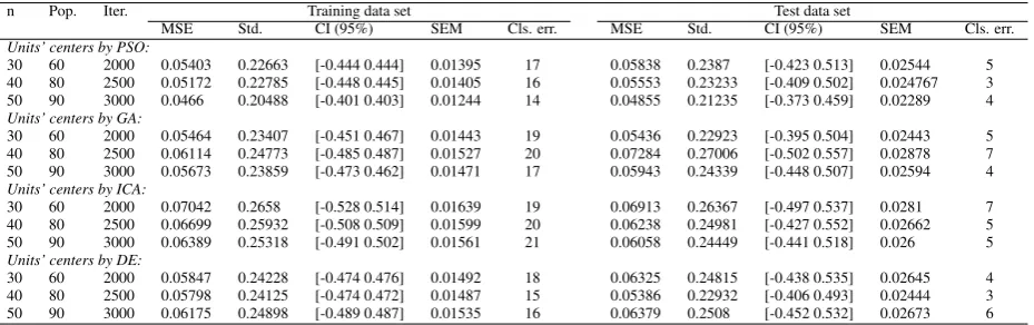
Table 8: Classification of Ionosphere data set based on RBF-PSO optimization algorithm
n Pop. Iter. Training data set Test data set
MSE Std. CI (95%) SEM Cls. err. MSE Std. CI (95%) SEM Cls. err. Units’ centers by PSO:
30 60 2000 0.05403 0.22663 [-0.444 0.444] 0.01395 17 0.05838 0.2387 [-0.423 0.513] 0.02544 5 40 80 2500 0.05172 0.22785 [-0.448 0.445] 0.01405 16 0.05553 0.23233 [-0.409 0.502] 0.024767 3 50 90 3000 0.0466 0.20488 [-0.401 0.403] 0.01244 14 0.04855 0.21235 [-0.373 0.459] 0.02289 4 Units’ centers by GA:
30 60 2000 0.05464 0.23407 [-0.451 0.467] 0.01443 19 0.05436 0.22923 [-0.395 0.504] 0.02443 5 40 80 2500 0.06114 0.24773 [-0.485 0.487] 0.01527 20 0.07284 0.27006 [-0.502 0.557] 0.02878 7 50 90 3000 0.05673 0.23859 [-0.473 0.462] 0.01471 17 0.05943 0.24339 [-0.448 0.507] 0.02594 4 Units’ centers by ICA:
30 60 2000 0.07042 0.2658 [-0.528 0.514] 0.01639 19 0.06913 0.26367 [-0.497 0.537] 0.0281 7 40 80 2500 0.06699 0.25932 [-0.508 0.509] 0.01599 20 0.06238 0.24981 [-0.427 0.552] 0.02662 5 50 90 3000 0.06389 0.25318 [-0.491 0.502] 0.01561 21 0.06058 0.24449 [-0.441 0.518] 0.026 5 Units’ centers by DE:
30 60 2000 0.05847 0.24228 [-0.474 0.476] 0.01492 18 0.06325 0.24815 [-0.438 0.535] 0.02645 4 40 80 2500 0.05798 0.24125 [-0.474 0.472] 0.01487 15 0.05386 0.22932 [-0.406 0.493] 0.02444 3 50 90 3000 0.06175 0.24898 [-0.489 0.487] 0.01535 16 0.06379 0.2508 [-0.452 0.532] 0.02673 6
Standard Error of Mean (SEM), Confidence Interval (CI) by 95% and the number of incorrect classifica-tion (Cls. err.). Firstly, we adjust RBF units’ cen-ters based on MSE as a frequently used cost function (minimization objective) in the literature. We employ four optimization algorithms which are widely used and
[image:10.595.68.533.492.638.2]Table 9: Classification of Zoo data set based on RBF-PSO optimization algorithm
n Pop. Iter. Training data set Test data set
MSE Std. CI (95%) SEM Cls. err. MSE Std. CI (95%) SEM Cls. err. Units’ centers by PSO:
30 50 2000 0.00156 0.03974 [-0.077 0.079] 0.00455 3 0.00394 0.0552 [-0.113 0.104] 0.01104 3 40 70 2500 0.00093 0.03024 [-0.059 0.059] 0.00366 1 0.00471 0.07 [-0.14 0.135] 0.01401 5 50 90 3000 0.00095 0.03114 [-0.061 0.061] 0.00335 3 0.00607 0.07197 [-0.157 0.131] 0.01439 4 Units’ centers by GA:
30 50 2000 0.00222 0.47477 [-0.093 0.094] 0.00544 4 0.00904 0.08952 [-0.212 0.139] 0.0179 7 40 70 2500 0.00141 0.03783 [-0.074 0.074] 0.00433 5 0.00595 0.07695 [-0.167 0.134] 0.01539 4 50 90 3000 0.00115 0.03422 [-0.067 0.067] 0.00392 4 0.00628 0.06858 [-0.147 0.122] 0.01383 4 Units’ centers by ICA:
30 50 2000 0.00211 0.04628 [-0.089 0.093] 0.0053 5 0.00706 0.08286 [-0.155 0.17] 0.01657 4 40 70 2500 0.0011 0.0334 [-0.065 0.066] 0.00383 2 0.00487 0.06209 [-0.155 0.17] 0.01241 6 50 90 3000 0.00102 0.03228 [-0.063 0.064] 0.0037 2 0.00826 0.08935 [-0.2 0.151] 0.01787 4 Units’ centers by DE:
30 50 2000 0.00159 0.04024 [-0.079 0.078] 0.00461 3 0.00514 0.07046 [-0.158 0.119] 0.01409 5 40 70 2500 0.00136 0.03712 [-0.073 0.073] 0.00425 4 0.00848 0.08664 [-0.206 0.134] 0.01733 6 50 90 3000 00113 0.03385 [-0.066 0.066] 0.00388 2 0.00635 0.074 [-0.155 0.135] 0.0148 4
[image:11.595.62.530.130.439.2](a) Multi objective (n=20) (b) Multi objective (n=40) (c) Multi objective (n=70)
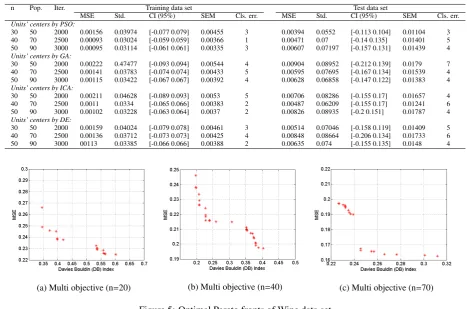
Figure 5: Optimal Pareto fronts of Wine data set
[image:11.595.79.516.463.590.2](a) Multi objective (n=20) (b) Multi objective (n=50) (c) Multi objective (n=70)
Figure 6: Optimal Pareto fronts of Iris data set
the optimal considered performance criteria. Tables 2-5 show the comparison of (best) results over applied benchmarking problems. As seen in these Tables, PSO performs better results in estimation of RBF units’ cen-ters as compared to others based on the applied perfor-mance measures. The second optimal results have also performed by GA. However, we have evaluated all re-sults as the (near) optimal adjustment of units’ centers
(a) Multi objective (n=60) (b) Multi objective (n=80) (c) Multi objective (n=90)
Figure 7: Optimal Pareto fronts of Ionosphere data set
(a) Multi objective (n=50) (b) Multi objective (n=70) (c) Multi objective (n=90)
Figure 8: Optimal Pareto fronts of Zoo data set
achieve better results than the other methods in terms of the classification error and other applied metrics. Ex-perimental results demonstrate that even though the ICA and the DE with not so proper results in obtaining RBF units’ centers could successfully provide low classifica-tion error. Unlike the suitable number of correct classifi-cation by ICA and DE, they do not usually perform well in terms of MSE, Std., CI (95%) and SEM as compared to PSO and GA. Since the number of correct classifica-tion is the major criterion in the classificaclassifica-tion problems, it can be concluded that the MSE (as minimization ob-jective) is not a suitable performance metric for finding the (near) optimal placement of units’ centers. To con-firm convincingly this claim, this paper presents a multi-objective approach to find the (near) optimal placement of centers. According to the first part of the proposed method (see Fig. 4), NSGA II was applied over bench-marking problems by two conflicting objectives (DBI and MSE) in order to find the well-separated centers and their local optimization, respectively. The experiment on proposed algorithm was repeated 5 times indepen-dently to find the optimal performance metrics. Figs. 5-8 are depicted the optimal Pareto front solutions of
(near) well-placed of RBF units’ centers through DBI (x-axis) and MSE (y-axis). We are going to show that for constructing final RBF neural networks, MSE is not solely the ideal accurate criterion.
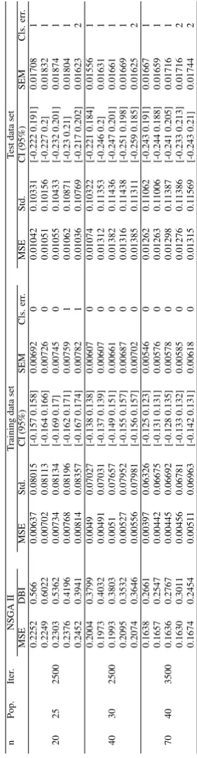
[image:12.595.86.516.284.408.2]T able 10: Classification of W ine data set based on proposed method n Pop. Iter . NSGA II T raining data set T est data set MSE DBI MSE Std. CI (95%) SEM Cls. err . MSE Std. CI (95%) SEM Cls. err . 0.2252 0.566 0.00637 0.08015 [-0.157 0.158] 0.00692 0 0.01042 0.10331 [-0.222 0.191] 0.01708 1 0.2249 0.6022 0.00702 0.08113 [-0.164 0.166] 0.00726 0 0.01051 0.10156 [-0.227 0.2] 0.01832 1 20 25 2500 0.2303 0.5362 0.00734 0.08134 [-0.169 0.17] 0.00745 0 0.01055 0.10433 [-0.232 0.201] 0.01874 1 0.2376 0.4196 0.00768 0.08196 [-0.162 0.171] 0.00759 1 0.01062 0.10871 [-0.23 0.21] 0.01804 1 0.2452 0.3941 0.00814 0.08357 [-0.167 0.174] 0.00782 1 0.01036 0.10769 [-0.217 0.202] 0.01623 2 0.2004 0.3799 0.0049 0.07027 [-0.138 0.138] 0.00607 0 0.01074 0.10322 [-0.221 0.184] 0.01556 1 0.1973 0.4032 0.00491 0.07031 [-0.137 0.139] 0.00607 0 0.01312 0.11353 [-0.246 0.2] 0.01631 1 40 30 2500 0.1993 0.3803 0.0051 0.07657 [-0.149 0.151] 0.00661 0 0.01382 0.11436 [-0.247 0.201] 0.01661 1 0.2095 0.3532 0.00527 0.07952 [-0.155 0.157] 0.00687 0 0.01316 0.11438 [-0.251 0.198] 0.01669 1 0.2074 0.3646 0.00556 0.07981 [-0.156 0.157] 0.00702 0 0.01385 0.11311 [-0.259 0.185] 0.01625 2 0.1638 0.2661 0.00397 0.06326 [-0.125 0.123] 0.00546 0 0.01262 0.11062 [-0.243 0.191] 0.01667 1 0.1657 0.2547 0.00442 0.06675 [-0.131 0.131] 0.00576 0 0.01263 0.11006 [-0.244 0.188] 0.01659 1 70 40 3500 0.1636 0.2767 0.00445 0.06692 [-0.128 0.135] 0.00578 0 0.01298 0.11387 [-0.241 0.205] 0.01716 1 0.1630 0.3011 0.00456 0.06781 [-0.133 0.132] 0.00585 0 0.01276 0.11386 [-0.233 0.213] 0.01716 2 0.1674 0.2454 0.00511 0.06963 [-0.142 0.131] 0.00618 0 0.01315 0.11569 [-0.243 0.21] 0.01744 2
the units’ centers in RBF networks. A new hybrid op-timization approach for well-separated centers (such as by DBI) and their local optimization (such as by MSE) in estimation of RBF units’ centers would fit consider-ably the performance requirements.
T able 11: Classification of Iris data set based on proposed method n Pop. Iter . NSGA II T raining data set T est data set MSE DBI MSE Std. CI (95%) SEM Cls. err . MSE Std. CI (95%) SEM Cls. err . 0.0136 0.2759 0.00465 0.06852 [-0.134 0.134] 0.00644 1 0.01183 0.10909 [-0.198 0.23] 0.01793 2 0.0129 0.0403 0.00527 0.07292 [-0.142 0.144] 0.00686 2 0.01285 0.10272 [-0.168 0.235] 0.02175 2 25 35 2500 0.0183 0.184 0.0055 0.07452 [-0 .145 0.147] 0.00701 1 0.01268 0.10028 [-0.173 0.22] 0.02106 2 0.0142 0.2386 0.00585 0.07486 [-0.15 0.151] 0.00723 1 0.00996 0.1012 [-0.197 0.2] 0.01663 2 0.0169 0.1924 0.00632 0.07488 [-0.156 0.157] 0.00751 2 0.01241 0.10918 [-0.191 0.237] 0.02148 2 0.0111 0.1911 0.00316 0.05651 [-0.111 0.111] 0.00531 1 0.01397 0.09296 [-0.153 0.191] 0.0205 1 0.0121 0.1752 0.00344 0.05893 [-0.115 0.116] 0.00554 1 0.01394 0.09134 [-0.146 0.212] 0.02005 1 35 50 3000 0.0106 0.2048 0.00346 0.05908 [-0.1 15 0.116] 0.00555 1 0.01362 0.09189 [-0.162 0.191] 0.02066 1 0.0116 0.1910 0.00377 0.06169 [-0.121 0.121] 0.0058 2 0.01295 0.09245 [-0.164 0.198] 0.02006 1 0.0105 0.2122 0.00381 0.06206 [-0.123 0.121] 0.00583 1 0.01241 0.09067 [-0.16 0.196] 0.02076 1 0.0095 0.1650 0.00416 0.06636 [-0.129 0.131] 0.00624 1 0.03992 0.05205 [-0.058 0.046] 0.0265 1 0.0088 0.1932 0.00418 0.06798 [-0.133 0.134] 0.00639 1 0.03904 0.05666 [-0.053 0.169] 0.02561 1 40 70 3500 0.0091 0.1744 0.0042 0.06814 [-0.1 33 0.135] 0.00641 1 0.03476 0.05989 [-0.074 0.161] 0.0245 1 0.0087 0.2108 0.00422 0.06829 [-0.132 0.135] 0.00642 1 0.03235 0.05287 [-0.056 0.152] 0.02335 1 0.0097 0.1636 0.00423 0.06903 [-0.134 0.136] 0.00649 2 0.03468 0.04836 [-0.045 0.144] 0.02425 1
10. Evaluation environment
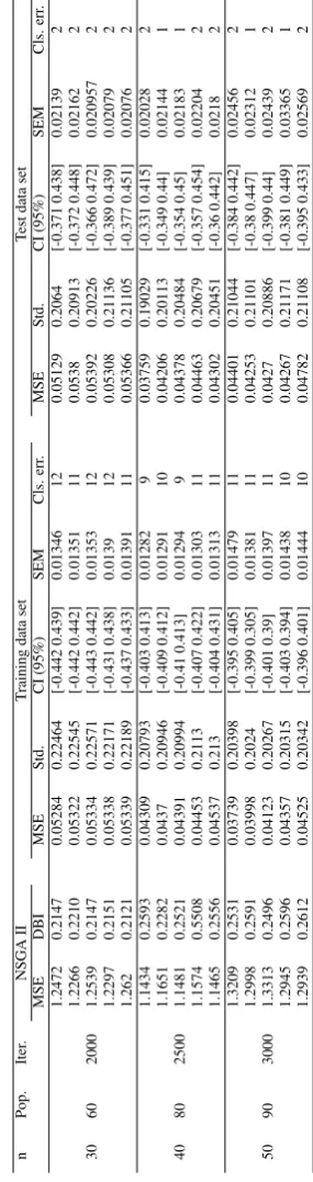
[image:13.595.360.499.79.626.2] [image:13.595.114.255.87.627.2]T able 12: Classification of Ionosphere data set based on proposed method n Pop. Iter . NSGA II T raining data set T est data set MSE DBI MSE Std. CI (95%) SEM Cls. err . MSE Std. CI (95%) SEM Cls. err . 1.2472 0.2147 0.05284 0.22464 [-0.442 0.439] 0.01346 12 0.05129 0.2064 [-0.371 0.438] 0.02139 2 1.2266 0.2210 0.05322 0.22545 [-0.442 0.442] 0.01351 11 0.0538 0.20913 [-0.372 0.448] 0.02162 2 30 60 2000 1.2539 0.2147 0.05334 0.22571 [-0.443 0.442] 0.01353 12 0.05392 0.20226 [-0.366 0.472] 0.020957 2 1.2297 0.2151 0.05338 0.22171 [-0.431 0.438] 0.0139 12 0.05308 0.21136 [-0.389 0.439] 0.02079 2 1.262 0.2121 0.05339 0.22189 [-0.437 0.433] 0.01391 11 0.05366 0.21105 [-0.377 0.451] 0.02076 2 1.1434 0.2593 0.04309 0.20793 [-0.403 0.413] 0.01282 9 0.03759 0.19029 [-0.331 0.415] 0.02028 2 1.1651 0.2282 0.0437 0.20946 [-0.409 0.412] 0.01291 10 0.04206 0.20113 [-0.349 0.44] 0.02144 1 40 80 2500 1.1481 0.2521 0.04391 0.20994 [-0.41 0.413] 0.01294 9 0.04378 0.20484 [-0.354 0.45] 0.02183 1 1.1574 0.5508 0.04453 0.2113 [-0.407 0.422] 0.01303 11 0.04463 0.20679 [-0.357 0.454] 0.02204 2 1.1465 0.2556 0.04537 0.213 [-0.404 0.431] 0.01313 11 0.04302 0.20451 [-0.36 0.442] 0.0218 2 1.3209 0.2531 0.03739 0.20398 [-0.395 0.405] 0.01479 11 0.04401 0.21044 [-0.384 0.442] 0.02456 2 1.2998 0.2591 0.03998 0.2024 [-0.399 0.305] 0.01381 11 0.04253 0.21101 [-0.38 0.447] 0.02312 1 50 90 3000 1.3313 0.2496 0.04123 0.20267 [-0.401 0.39] 0.01397 11 0.0427 0.20886 [-0.399 0.44] 0.02439 2 1.2945 0.2596 0.04357 0.20315 [-0.403 0.394] 0.01438 10 0.04267 0.21171 [-0.381 0.449] 0.03365 1 1.2939 0.2612 0.04525 0.20342 [-0.396 0.401] 0.01444 10 0.04782 0.21108 [-0.395 0.433] 0.02569 2
for evaluating the performance of considered mitiga-tion method. ndnSIM simulamitiga-tion environment repro-duces the basic structures of a NDN node (i.e., CS, PIT, FIB, strategy layer, and so on). The proposed detec-tion method (first phase) was implemented by the MAT-LAB software on the Intel Pentium 2.13 GHz CPU, 4 GB RAM running Windows 7 Ultimate. This algorithm
T able 13: Classification of Zoo data set based on proposed method n Pop. Iter . NSGA II T raining data set T est data set MSE DBI MSE Std. CI (95%) SEM Cls. err . MSE Std. CI (95%) SEM Cls. err . 0.7917 0.3458 0.00051 0.02279 [-0.044 0.045] 0.00261 0 0.00382 0.05222 [-0.132 0.073] 0.01204 1 0.7954 0.3307 0.00057 0.02405 [-0.047 0.047] 0.00275 1 0.0035 0.05126 [-0.126 0.075] 0.01125 1 50 40 3000 0.826 0.3252 0.00058 0.02443 [-0.0 48 0.049] 0.0028 1 0.00333 0.05226 [-0.113 0.092] 0.01021 1 0.793 0.3429 0.00066 0.02602 [-0.051 0.051] 0.00298 0 0.00307 0.05212 [-0.11 0.094] 0.01182 1 0.8924 0.3111 0.00087 0.02981 [-0.059 0.058] 0.00318 1 0.00318 0.05272 [-0.092 0.115] 0.01004 2 0.7185 0.3212 0.00047 0.02188 [-0.042 0.044] 0.0025 0 0.00451 0.06023 [-0.104 0.132] 0.01164 1 0.747 0.2903 0.00076 0.02783 [-0.054 0.055] 0.00319 0 0.00413 0.05987 [-0.121 0.114] 0.01097 2 70 50 3000 0.7383 0.2911 0.00082 0.02895 [-0.0 57 0.057] 0.00332 1 0.00304 0.05631 [-0.112 0.108] 0.01126 2 0.7081 0.239 0.00083 0.0291 [-0.056 0.058] 0.00333 0 0.00439 0.06055 [-0.123 0.115] 0.01151 1 0.7482 0.2816 0.00085 0.02946 [-0.058 0.058] 0.00338 1 0.0029 0.05502 [-0.108 0.107] 0.011 2 0.6831 0.2927 0.00049 0.02233 [-0.044 0.044] 0.00256 0 0.00555 0.06215 [-0.142 0.102] 0.01613 2 0.6834 0.2508 0.00043 0.021 [-0.041 0.041] 0.0024 0 0.00591 0.06015 [-0.135 0.101] 0.01123 2 90 60 3000 0.6969 0.1378 0.00065 0.0258 [-0.0 5 0.051] 0.00296 0 0.00608 0.06658 [-0.142 0.119] 0.01129 2 0.7113 0.1317 0.00078 0.02823 [-0.055 0.056] 0.00323 1 0.00587 0.06653 [-0.146 0.115] 0.0113 2 0.7246 0.1221 0.00028 0.01711 [-0.033 0.034] 0.00196 0 0.00261 0.0516 [-0.109 0.094] 0.01032 1
[image:14.595.360.500.80.627.2] [image:14.595.112.255.88.628.2]consider-ably applied performance metrics as compared to two recently applied DoS attack mitigation methods namely satisfaction-based pushback and satisfaction-based In-terest acceptance [15]. We perform 10 times simulation runs to calculate the average performance metrics. Our experiments are performed over two topologies shown in Figs. 9 and 10. Fig. 9 corresponds to DFN-like (Deutsche Forschungsnetz as the German Research Network) [100], and Fig. 10 corresponds to the AT&T network [101]. We use the symbols Cx, Px, Rx, and Ax
to representx-th consumer, producer, router and adver-sary nodes, respectively. In spite of various arguments and experiments, there is no typically and properly jus-tification for NDN parameters and they have specified based on authors’ experiences and designs [2]. The experimental setup (i.e., attack and non-attack traffics modeling) is performed over two applied topologies as follows. For attack effectiveness, we examine the per-formance of the network’s data packet delivery and sat-isfied Interest rate under the different scenarios (see DoS attacks issues in section 3):
1. Interest flooding attack (dynamically-generated In-terest packets) for the existent Data.
2. Interest flooding (dynamically-generated Interest packets) for the non-existent Data. It can be in the form of brute-force attack (very high distribution of Interest) or normal distribution of Interest. 3. Hijacking, in which a producer silently drops all
incoming Interest traffic in downstream interfaces. 4. Content poisoning (bogus data packets), in which a producer deliberately signs data packets with a wrong key. We assume that the routers firstly check the signature filed of data packet, then cache and route the packet toward its destination if the signa-ture is valid. Hence, the bogus data packets cannot be cached in the intermediate routers.
[image:15.595.338.502.109.292.2]In our configurations, we set nodes’ PIT size to 120 KB, while the Interest expiration time was set to the default timeout of 4 sec. We set the link delay and queue length parameters to fixed values for every node in the simulated topologies. In particular, we set delay and queue length to 10 ms and 400 for both considered topologies, respectively. The PIT entries replacement policy was adopted to the least-recently-used (the old-est entry with minimum number of incoming faces will be removed if PIT size reached its limit) as a widely used strategy. The nodes’ cache capacity was set to 1000 contents and cache replacement policy was set to least-recently-used method. The other system settings of investigated network topologies are summarized in Table 14. As shown in this table, we ran various traffic
Figure 9: DFN-like topology
patterns in which each configuration changes in every 10 simulation runs in order to perform different network characteristics.
We first analyze the topologies without any adversarial traffic, then with adversarial traffic, finally considera-tion of the proposed mitigaconsidera-tion method over the illegit-imate traffics. Our assumption is that, the behavior of legitimate (honest) consumers is unchanged in duration of the simulation, and the adversary is not allowed to control routers. To study the performance of our pro-posed countermeasure algorithm under range of condi-tions, we varied the percentage of attackers and their run times in the considered topologies in Table 14.
11. The proposed countermeasure: proactive detec-tion and adaptive reacdetec-tion
In this section, we introduce our method, a two phases -detection and reaction- framework for mitigat-ing DoS attacks in NDN.
11.1. Detection Phase
This step adopts our proposed intelligent classifier from section 8.1. We choose the DFN-like topology (Fig. 9) in the training phase with the recommended pa-rameter settings in Table 14. We then apply this trained network for the detection purposes in both DFN-like and AT&T topologies.
Figure 10: AT&T topology
Table 14: Network parameters considered
Node Distribution Pattern Frequency Run time (minute) Producer Goal DFN-like topology (Fig. 9)
C1 randomize uniform [100 500] 0-40 P1 normal
C2 randomize exponential [100 500] 2-40 P2 normal
C3 Zipf-Mandelbort (α=[0.5 0.9]) exponential [100 500] 3-40 P3 normal
C4 randomize uniform [100 500] 4-40 P6 normal
C5 Zipf-Mandelbort (α=[0.5 0.9]) exponential [100 500] 3-40 P2, P3 normal
C6 randomize uniform [100 500] 5-40 P3 normal
C7 randomize uniform [100 500] 7-16, 22-31 P6, P4 sign data with the wrong key C8 randomize exponential [100 500] 8-18, 25-40 P1 normal
A1 randomize uniform [1500 3000] 7-16 P1 Interest flooding for existence data A2 Zipf-Mandelbort (α=[0.5 0.9]) uniform [1500 3000] 22-31 no producer Interest flooding for non-existence data A3 randomize uniform [400 800] 7-16 P5 (hijacker) hijacking incoming Interest packets A4 randomize exponential [1500 3000] 22-31 P6 Interest flooding for existence data AT&T topology (Fig. 10)
C0, C7 randomize uniform [200 600] 0-50 P0, P1 normal
C1, C8 randomize exponential [200 600] 2-50 P0 normal
C2, C9 randomize exponential [200 600] 3-50 P1 normal
C3, C10 randomize uniform [200 600] 4-50 P1 normal
C4, C11 Zipf-Mandelbort (α=[0.5 0.9]) exponential [200 600] 5-50 P0, P1 normal C5, C12, C13 randomize uniform [200 600] 6-50 P0, P1 normal
C6, C14, C15 randomize uniform [200 600] 8-50 P1 normal
A0 randomize uniform [1000 3000] 7-25 P1 Interest flooding for existence data A0 randomize exponential [1000 3000] 30-45 P1 Interest flooding for existence data A1 Zipf-Mandelbort (α=[0.5 0.9]) exponential [500 1000] 7-25 P0 sign data with the wrong key A1 Zipf-Mandelbort (α=[0.5 0.9]) uniform [1000 3000] 30-45 no producer Interest flooding for non-existence data A2 randomize exponential [1000 3000] 7-25 no producer Interest flooding for non-existence data A2 randomize uniform [1000 3000] 30-45 P1 Interest flooding for existence data
namespace. The proper combining/choosing of statis-tic parameters in NDN routers for maximum eff ective-ness against attacks and anomalies, minimum disorder-ing of legitimate traffics, and distinguishing between ’good’ and ’bad’ Interest packets are research chal-lenges [15, 20]. Hence, we employed simple intrin-sic features from the network which is shown in Table 15 (i.e., the input features in the RBF neural network). In the training process, all the features beginning with
[image:16.595.68.540.374.604.2]be satisfied with the same Data. Hence, if a number of In/Out Data be more than the In/Out satisfied Inter-est for a given interface or vice versa, it would not be a misbehaving. Another instance is that, Interest packets from a consumer are possible to arrive to several routers and perhaps several producers that can satisfy the In-terests. Corresponding data packet will send back from producer(s). A router in the middle way, receives the first packet from any producer and will forward it to the consumer and remove the PIT entry. When the second Data object arrives to the router, it will be discarded by the routers as unsolicited. Hence, it is more likely that a rate of In/Out Data or DropData be more than In/Out Interest rate and vice versa in a corresponding interface. Obviously, it is not an attack or anomaly behavior. Also, in a given interface, the rate of the InInterest may be less that the SatisfiedInterest rate which in due to the portion of the satisfaction rate comes from the previous time in-terval. On the other hand, the rate of the OutData may be more than the InInterest rate, which is for routing the cached data for satisfying incoming Interest packets. To sum up, different parameters mentioned by our detec-tion module act as weights and counterweights for mis-behaving consumer and producer detection purposes. For constructing a predictor module based on the RBF neural network, at first the centers, widths and weights are computed and adjusted using training set 75% of data set, and then the remaining part of the data set as the test set, is used to validate the trained network func-tionality. We trained and evaluated the network with various number of RBF units, where the three optimal results are summarized in Table 16. The optimal Pareto front solutions by NSGA II are also depicted in Fig. 11. We computed the MSE, Std., CI (95%), SEM and classification error for both training and testing parts. The histogram analysis of the classification error dis-tribution and the regression analysis of the misclassifi-cation are shown in Figs. 12 and 13, respectively. As seen in these Figures and Table 16, third parameter set-tings could provide the better results as compared to the two others in terms of the applied performance metrics. Hence, these (near) optimal parameter settings are used to construct our RBF classifier (predictor).
As we expected (based on our proof in section 9), This phase constructs an optimized and more accurate RBF classifier (predictor) for our DoS attack mitigation pur-poses in NDN. According to the traffic flows type in the training data set (see Table 14), this predictor learned three types of traffic patterns including normal, mali-cious behavior from consumers and producers. This predictor module runs on routers, in order to continu-ously monitor per-interface required statistical
[image:17.595.314.524.208.508.2]informa-tion. This module is executed at fixed time intervals -typically every 0.5 sec - to provide a proactive detec-tion behavior. Finally, based on three types of predic-tion (normal, misbehaving consumer and misbehaving producer), we should respond an appropriate action as detailed in the next subsection.
Table 15: Feature construction
Feature Description
InInterests a number of arrival Interest in an interface InData a number of arrival data in an interface InSatisfiedInterests a number of satisfied Interests where
interface was part of the incoming set InTimedOutInterests a number of timed out Interests where interface was part of the incoming set OutInterests a number of sent Interest from an interface OutData a number of sent data from an interface OutSatisfiedInterests a number of satisfied Interests where
interface was part of the outgoing set OutTimedOutInterests a number of timed out Interests where
[image:17.595.314.527.214.353.2]interface was part of the outgoing set DropInterests a number of dropped Interest in an interface DropData a number of dropped data in an interface SatisfiedInterests a total number of satisfied Interests TimedOutInterests a total number of timed out Interests
Figure 11: Optimal Pareto fronts of DFN-like training phase
11.2. Reaction Phase
de-(a) 1st histogram (b) 2nd histogram (c) 3rd histogram
Figure 12: The histogram analysis of the classification error distribution in DFN-like topology
[image:18.595.76.511.284.450.2](a) 1st Regression (94.97%) (b) 2nd Regression (94.96%) (c) 3rd Regression (95.18%)
Figure 13: Regression of the classification error between target and predicted output in DFN-like topology
tector module reports the normal traffic in the next time interval.
Figure 14: unsatisfied-based pushback example
11.2.1. reaction regarding to misbehaving consumer
When the proposed intelligent detector module in router detects adversarial traffics from a set of interfaces, it sends an alert message on each of them. An alert message is an unsolicited content
packet which belongs to a reserved namespace
(”/pushbackmessage/alert/”) in our
implementa-tion. There are two reasons for using content packet rather than Interest packet for carrying pushback message [11]:
1. during an attack, the PIT of next hop connected to the offending interface may be full, and therefore the alert message may be discarded, and
2. content packets are signed, while Interests are not. This allows routers to receive the content packets as a legitimate packet for processing.
[image:18.595.72.282.527.618.2](neigh-T
able
16:
Classification
of
NDN
data
set
based
on
proposed
method
n
Pop.
Iter
.
NSGA
II
T
raining
data
set
T
est
data
set
MSE
DBI
MSE
Std.
CI
(95%)
SEM
Cls.
err
.
MSE
Std.
CI
(95%)
SEM
Cls.
err
.
0.0314
0.0979
0.00998
0.09983
[-0.192
0.197]
0.00555
2
0.02354
0.15414
[-0.301
0.304]
0.01476
3
80
40
2500
0.0643
0.0979
0.00994
0.09986
[-0.186
0.206]
0.00555
2
0.02486
0.15841
[-0.324
0.297]
0.01517
3
0.0315
0.0914
0.00952
0.09505
[-0.187
0.186]
0.00543
1
0.02311
0.15271
[-0.299
0.3]
0.01421
1
bor node). Also, an unsatisfied rate is 50% foreth0
and 70% foreth1. Our proposed reaction mechanism is as follows:
1. RouterCwill send a pushback alert message to the neighbors frometh0andeth1.
2. Routers A and B, after receiving alert mes-sage from C will readjust their local
inter-faces limit to ’announced reduced rate’ ×
’local unsatisfied rate’in each local
face. If the new limit in the corresponding inter-face exceeds the predefined threshold φ, the cor-responding interface gets new reduction of Inter-est rate in downstream. For instance, we assume
φ=5% so that routerBdecreases the Interest rate of eth0to 50% andeth1 to 15%. RouterA de-creases the Interest rate in its three interfaces to 63%, 0 (the new limit rate (=3.5%) is under pre-defined threshold (=5%) and will not be changed) and 28% in eth0, eth1 and eth2, respectively. This threshold allows bandwidth usage be con-sumed for legitimate traffics in the nearest next time interval and intensifies Interest rate reduction for adversaries in each next time intervals. 3. Our wait time strategy for the reduction period in
neighbor nodes is an ascending penalty. If in a time intervaltin interfacejthe misbehaving traf-fic be reported, a counter sets to 1 sec. If in the next time interval t+1 the misbehaving again be reported, a counter sets to 2 sec. Our ascending penalty method is in 2counter. Initially,counter=0
and increase linearly in each time interval. The counter is set to the initial value when there is no misbehaving prediction in the next time interval. This ascending penalty intensifies the penalty for adversaries and alleviates the bandwidth usage for legitimate (honest) users.
4. Any neighbor node may obey (ignore) the an-nounced limit rate and send Interest packets with-out any restriction from the upstream interface. Our algorithm after twice refusing the alert mes-sage will band the incoming Interest packets from the corresponding interface for a long time period.
At the next iteration of the unsatisfied-based pushback mechanism, legitimate user(s) will be able to gradu-ally improve their satisfaction rate and sending Interest packets on both routerAandB. After applying the alert message in routerA, the Interest rate of the adversary will be decreased to around 63% in the next iteration. It allows bandwidth usage be consumed for 2nd legiti-mate user, that it will considerably led to the increasing of legitimate Interests rate. If the adversary continues its misbehaving in the next times, the ascending wait time strategy will increase the penalty rate of the illegal Inter-est packets. Hence,eth1andeth2interfaces in router
Awill get through and return Data, eventually resulting in a full allowance in the link between the routersAand
C.
[image:19.595.165.209.87.631.2]mechanism is shown in Algorithm 1. In this algo-rithm, theDecreasefunction decreases the Interest rate from corresponding interface with announced param-eters. After normal traffic prediction, the Increase
function sets the default Interest rate on the correspond-ing interface in the next time interval. The IsFresh
function checks the freshness of the alert message when there is no previously alert message.
Input:AlertMsg,timestampof alert generation,reduced rateandwait timefrom interfacejin routeri(rij)
Result: (1) adaptive pushback reaction and (2) pushback alert message generation
1 counterj=0// initial counter for generating wait
time in interface j
2 φ=5%// reduction threshold of Interest rate
/* section: adaptive pushback reaction */
3 ifAlertMsgisPushback alert messagethen
4 ifVerify(AlertMsg.signature)and
IsFresh(AlertMsg.timestamp)then
/* Pushback reaction */
5 foreachlocal interface jdo
6 new rate=unsatisfied rate of j×
announced reduced rate;
7 ifφ <new ratethen
/* intensify the penalty */
8 Decrease(interface j,new rate, announced wait time);
9 else
/* reset to original setting */
10 Increase(interface j,original rate);
11 else
12 Drop(AlertMsg);
13 return ;
/* section: Pushback alert message generation */
14 if(predictor module reports theadversary consumer
(neighbor)in local interface j)then
15 if(time from last sentAlertMsgto local interface rij<
current local time)then
/* Pushback alert message generation */
16 new time interval=2counterj;
17 AlertMsg=(currenttimestampof alert generation, currentunsatisfied ratein local interfacej, new time interval);
18 Send(AlertMsgto rij);
19 counterj=counterj+1;
20 else
/* reset to original setting */
21 counterj=0 ;
22 Increase(interface j,original rate);
Algorithm 1: Unsatisfied-based pushback algo-rithm
11.2.2. reaction regarding to misbehaving producer
If the predictor module predicts a misbehaving pro-ducer from an interfacej, we build an adaptive and sim-ple forwarding strategy. The main goal is to retrieve data via the best performance path(s), and to quickly re-cover packet delivery problem by the other (possible) le-gitimate producers. When a predictor module in a router
ireports a misbehaving producer in an interfacej, the in-terface status changes to theunavailable(can not bring data back) and will be deactivated for a predefined time interval. This type of forwarding strategy can increase the data retrieving chance for awaiting Interest packets in the PIT table by changing the forwarding path. We apply the wait time strategy from the misbehaving con-sumer section (see section 11.2.1). After normal pre-diction in the next time intervals, the interface status changes to available(can bring data back). It means, it is ready for forwarding Interest packets via this inter-face. It is expected that in the next time intervals, when there is no any legitimate producer to satisfy the corre-sponding Interest packets in an interfacej, the predictor module reports misbehaving consumer (neighbor) from upstream interfacej, where Interest packets are suscep-tible to be illegal traffics. Then, the rate of incoming Interest packets should gradually decrease in upstream interfacej based on our ascending penalty mechanism in previous subsection.
12. Experimental results and evaluation
In this section we report the experimental evaluation of countermeasures presented in Section 11. Our coun-termeasures are tested over two considered topologies in Figs. 9 and 10. Each router implements the proposed detection technique discussed in Section 11.1 and adap-tive reaction technique discussed in 11.2.
We report the results based on the five conditions: base-line, attack (no countermeasure), our proposed method, and two DoS mitigation methods applied in this work including based pushback and satisfaction-based Interest acceptance from [15]. Figs. 15 and 18 show the average Interest satisfaction ratio for le-gitimate users within 10 runs in DFN-like and AT&T topologies, respectively. Our results show that the pro-posed intelligent hybrid algorithm (proactive detection and adaptive reaction) is very effective for shutting down the adversary traffics and preventing legitimate users from service degradation by the accuracy more than 90% during the attack.
Figure 15: Interest satisfaction ratio for legitimate users in DFN
Figure 16: PIT usage with countermeasures in DFN
[image:21.595.147.452.533.684.2]Figure 18: Interest satisfaction ratio for legitimate users in AT&T
Figure 19: PIT usage with countermeasures in AT&T
[image:22.595.147.451.530.684.2]![Figure 1: CCN packet types [12]](https://thumb-us.123doks.com/thumbv2/123dok_us/435420.1043079/3.595.82.269.395.472/figure-ccn-packet-types.webp)