R E S E A R C H
Open Access
Extragradient thresholding methods for
sparse solutions of co-coercive NCPs
Meijuan Shang
1,2*, Shenglong Zhou
3and Naihua Xiu
1*Correspondence:
[email protected] 1Department of Applied
Mathematics, Beijing Jiaotong University, Beijing, 100044, P.R. China 2Department of Mathematics,
Shijiazhuang University, Shijiazhuang, 050035, P.R. China Full list of author information is available at the end of the article
Abstract
In this paper, we aim to find sparse solutions of co-coercive nonlinear
complementarity problems (NCPs). Mathematically, the underlying model is NP-hard in general. Thus an
1regularized projection minimization model is proposed for
relaxation and an extragradient thresholding algorithm (ETA) is then designed for this regularized model. Furthermore, we analyze the convergence of this algorithm and show any cluster point of the sequence generated by ETA is a solution of NCP. Numerical results demonstrate that the ETA can effectively solve the
1regularized
model and output very sparse solutions of co-coercive NCPs with high quality. MSC: 90C33; 90C26; 90C90
Keywords: nonlinear complementarity problems; sparse solution; co-coercive;
1relaxation; extragradient; convergence
1 Introduction
The nonlinear complementarity problem, denoted by theNCP(F), is to find a vectorx∈Rn such that
x≥, F(x)≥, xF(x) = ,
whereFis a mapping fromRninto itself. The set of solutions to this problem is denoted bySOL(F). Throughout this paper, we assumeSOL(F)=∅.
NCPs have various important applications in economics and engineering, such as Nash equilibrium problems, traffic equilibrium problems, contact mechanics problems, option pricing. Extensive studies of NCPs have been done; see [–] and the references therein. Numerical methods for solving NCPs, such as filter method, continuation method, non-smooth Newton’s method, non-smoothing Newton methods, Levenberg-Marquardt method, projection method, descent method, interior-point method have been extensively inves-tigated in the literature. However, it seems that there is a vacant study of sparse solutions for NCPs. In fact, in real applications, it is very necessary to investigate the sparse solution of the NCPs. For example this is so in bimatrix games [] and portfolio selections []. For more details, see [].
In this paper, we try to compute a sparse solution of theNCP(F), which has the smallest number of nonzero entries. To be specific, we seek a vectorx∈Rnby solving the
-norm
minimization problem
minx
s.t. x≥,F(x)≥,xF(x) = , ()
wherexstands for the number of nonzero components ofx. A solution of () is called
the sparse solution ofNCP(F).
The above minimization problem () is in fact a sparse optimization [–] with equi-librium constraints. In the view of the objection function, the problem is-norm
mini-mization problem, which is combinatorial and generally NP-hard. From the point of view of constraint conditions, it is in fact a mathematical program with equilibrium constraints (MPEC) [–]. It is not easy to get solutions due to the equilibrium constraints, even for a continuous objective function.
To overcome the difficulty for the-norm, many researchers have suggested to relax
the norm and, instead, to consider the norm; see [, , –]. Motivated by this
outstanding work, we consider applyingnorm minimization to find the sparse solution
of NCPs, and we obtain the following minimization problem to approximate ():
min x∈Rnx
s.t. x≥,F(x)≥,xF(x) = , ()
wherex=
n i=|xi|.
To overcome the difficulty for the complementarity constraint, we make use of theC -function Fmin(x) to construct the penalty of violating the complementarity constraints. TheC-function Fminassociated with the ‘min’ function can be given by
Fmin(x) =x–Rn
+
x–F(x)x–x–F(x)+, () whereFis a mapping fromRninto itself, and
Rn
+ is the Euclidean metric projector onto
the nonnegative orthant.
It is well known [] that solvingNCP(F) is equivalent to solving the fixed point equation
Fmin(x) = , that is,
x∈SOL(F) ⇔ x=x–F(x)+, ()
where [·]+is the Euclidean metric projector onto the nonnegative orthant.
Combining () and (), by introducing a new variablez∈Rn, we obtain the following regularized minimization problem:
min
x,z∈Rnfλ(x,z) :=x–z
+λx
s.t. z=x–F(x)+, ()
whereλ> is a regularization parameter and · is denoted as the Euclidean norm. We call () theregularized projection minimization problem.
This paper is organized as follows. In Section , we approximate () by the
good approximation. In Section , we propose an extragradient thresholding algorithm (ETA) for () and also analyze the convergence of this algorithm. Numerical results are demonstrated in Section to show that () is promising in providing a sparse solution of co-coercive NCPs.
2 The
1regularized approximation
In this section, we study the relation between the solutions of model () and those of model ().
Theorem . For any fixedλ> ,the solution set of()is nonempty and bounded.Let
{(xλk,zλk)}be a solution of(),and{λk}be any positive sequence converging to.IfSOL(F)=
∅,then{(xλk,zλk)}has at least one accumulation point,and any accumulation point x ∗of
{xλk}is a solution of().
Proof For any fixedλ> , it is easy to show the coercivity offλ(x,z) in (), namely
fλ(x,z)→+∞ as(x,z)→ ∞. ()
We also note that for anyx∈Rnandz∈Rn,fλ(x,z)≥. This together with () implies the level set
L= (x,z)∈Rn×Rn|fλ(x,z)≤fλ(x,z) andz=
x–F(x)+
is nonempty and compact, wherex∈Rnandz= [x–F(x)]+ are given points. The
solution set of () is nonempty and bounded sincefλ(x,z) is continuous onL.
Now we show the second part of this theorem. Letx∈SOL(F) andz= [x–F(x)]+. From
(), we havex=z. Since (xλk,zλk) is a solution of () withλ=λk, wherezλk= [xλk–F(xλk)]+, it follows that
max xλk–zλk,λkxλk
≤ xλk–zλk+λkxλk
≤ x–z+λkx
=λkx. ()
From the above inequality, we derive that, for anyλk> ,
xλk≤ x. ()
Hence the sequence{xλk} is bounded and has at least one cluster point. Note that the sequence{zλk}is also bounded becausexλk–zλk≤λkx≤λx(λk→).
Letx∗andz∗ be any cluster points of{xλk}and{zλk}, respectively. Then there exists a subsequence of{λk}, say{λkj}, such that
lim kj→∞
xλkj=x∗ and lim kj→∞
We can obtainz∗= [x∗–F(x∗)]+by lettingkjtend to∞inzλkj = [xλkj –F(xλkj)]+. Letting
λkj tend to in
xλkj –zλkj≤λkjx
yieldsx∗=z∗. Consequently,x∗= [x∗–F(x∗)]+follows, which manifestsx∗∈SOL(F). From
(), namelyxλkj≤ x,kjtending to∞, we getx∗≤ x. Then by the arbitrariness
ofx∈SOL(F), we knowx∗is a solution of problem (). This completes the proof.
3 Algorithm and convergence
In this section, we suggest the extragradient thresholding algorithm (ETA) to solve
regu-larization projection minimization problem () and give the convergence analysis of ETA. First we state some basic operator concepts as regards monotonicity and some proper-ties of the projection operator. LetPK(·) denote the projection operator fromRnontoK, a nonempty closed convex subset ofRn. From the definition of projection operator, it fol-lows that
y–PK(x),PK(x) –x
≥, ∀y∈K,x∈Rn. ()
Consequently, we have
PK(x) –PK(y),x–y≥PK(x) –PK(y), ∀x,y∈Rn, ()
PK(x) –PK(y)≤ x–y, ∀x,y∈Rn, ()
PK(x) –y≤ x–y–PK(x) –x, ∀y∈K,x∈Rn. ()
Lemma .[] Define a residue function
e(x,α) =x–PKx–αF(x), α≥.
The following statements are valid.
(a) ∀α> ,F(x)e(x,α)≥e(xα,α); (b) for anyα> , e(xα,α) is non-increasing;
(c) for anyα≥,e(x,α)is non-decreasing.
In this paper, we suppose the mappingF:Rn→Rnis co-coercive on a subset K ofRn. That is, there exists a constantc> such that
F(x) –F(y),x–y≥cF(x) –F(y), ∀x,y∈K. It is clear that the co-coercive mapping is monotone, namely,
F(x) –F(y),x–y≥, ∀x,y∈K,
but not necessarily strongly monotone,i.e., there is a constantc> such that
Remark . Every affine monotone function which is also symmetric must be co-coercive (onRn). The Euclidean projectorPKandI–PKare both ‘co-coercive‘ functions [, ].
Lemma . Suppose that F(·)is co-coercive on K with modulus c> .Then for any given positive real numberα,when c>α/,the operator I–αF is nonexpansive,that is,for any x,y∈K,
(I–αF)(x) – (I–αF)(y)≤ x–y.
Proof For anyx,y∈K, whenc>α/, using the co-coercivity ofF, it follows that
(I–αF)(x) – (I–αF)(y)
=(x–y) –αF(x) –F(y)
=x–y– αx–y,F(x) –F(y)+αF(x) –F(y)
≤ x–y–α(c–α)F(x) –F(y)
≤ x–y,
which showsI–αFis nonexpansive.
For givingzk∈Rn
+andλk> , we consider an unconstrained minimization subproblem: min
x∈Rnfλk
x,zk:=x–zk+λkx. ()
Evidently, the minimizerxsof the model () must satisfy the corresponding optimality condition
xs=Sλk
zk, ()
where the shrinkage operatorSλis defined by
Sλ(z)i=
zi–λ, zi≥λ,
, ≤zi<λ. ()
Evidently, the shrinkage operatorSλis component-wise,i.e., (Sλ(z))i=Sλ(zi). Moreover, it is nonexpansive;i.e.,Sλ(x) –Sλ(y) ≤ x–y, for anyx,y∈Rn
+, see []. It demonstrates
that a solutionx∈Rnof the subproblem () can be analytically expressed by (). By the solution representation, we construct the following extragradient thresholding algorithm (ETA) to solve theregularized projection minimization problem ().
Input:c-the co-coercive modulus ofF. Step :Choose=z∈Rn
+,λ,β> ,τ,γ,μ∈(, ),βγ< c, > and integers
nmax>K> . Setk= .
Step :Compute
xk=Sλk
zk,
whereαk=βγmk withmkbeing the smallest nonnegative integer satisfying
Fxk–Fyk≤μx
k–yk
αk
. ()
Step :Ifxk–zk ≤ or the number of iterations is greater thann
max, then return zk,xk,ykand stop. Otherwise, compute
zk+=xk–αkFyk+
and updateλk+by
λk+=
τ λk, ifk+ is a multiple ofK,
λk, otherwise,
andk=k+ , then go to Step.
Before analyzing the convergence of ETA, we first present a key lemma as regards co-coercive mapping.
Lemma . Suppose that mapping F is co-coercive andSOL(F)=∅.If xkgenerated by ETA is not a solution ofNCP(F),then for anyx∈SOL(F),we have
Fyk,xk–x≥Fyk,xk–yk≥( –μ)x k–yk
β . ()
Proof For anyx∈SOL(F), we haveF(x)x= . Sinceyk∈Rn
+, it follows thatF(x),yk–x ≥
. It is clear that the co-coercive mapping is pseudo-monotone, that is,
x–y,F(y)≥ ⇒ x–y,F(x)≥, ∀x,y∈Kandx=y.
By the definition of pseudo-monotonicity, it follows thatF(yk),yk–x ≥. Hence,
Fyk,xk–x=Fyk,xk–yk+yk–x
≥Fyk,xk–yk
=Fxk,xk–yk–Fxk–Fyk,xk–yk
≥
αk
xk–yk– μ
αk
xk–yk
≥ –μ
β x
k–yk
,
where the last inequality but one follows from Lemma . and ().
We now begin to analyze the convergence of the proposed ETA.
Theorem . Suppose that the mapping F is co-coercive with modulus c>βγ/ and SOL(F)=∅.Let{(zk,xk,yk)}and{λ
k}be sequences generated by ETA,then
(i) the sequences{zk},{xk},and{yk}are all bounded;
Proof (i) Letx∈SOL(F). By the definition () of operatorSλ, we have
xk–x=S λ
zk–x≤zk–x+√nλk/≤zk–x+
√
nλ/. ()
In view ofx∈SOL(F), we havex= [x–αkF(x)]+. Sincec>βγ/ >αk/, by Lemma ., we see thatI–αkFis nonexpansive. Together with the nonexpansive property of the projec-tion operator, it follows that
yk–x=xk–αkF
xk+–x
=xk–αkFxk+–x–αkF(x)+
≤(I–αkF)xk–x
≤xk–x
≤zk–x+√nλk/
≤zk–x+√nλ
/. ()
From () and (), we obtain
zk+–x =xk–αkFyk+–x
≤xk–αkFyk–x–zk+–xk+αkFyk =xk–x– αk
Fyk,zk+–x–zk+–xk
≤xk–x– α k
Fyk,zk+–yk–zk+–xk =xk–x–zk+–yk–yk–xk
+ xk–yk–αkFyk,zk+–yk. ()
Byyk= [xk–αkF(xk)]+and (), it follows that
xk–yk–αkF
yk,zk+–yk
≤xk–yk–α kF
yk,zk+–yk+ yk–xk+α kF
xk,zk+–yk = αk
Fxk–Fyk,zk+–yk
≤αkFxk–Fyk+zk+–yk. ()
Replacing () into (), by () and (), we deduce
zk+–x
≤xk–x–yk–xk+αkFxk–Fyk
≤xk–x–yk–xk+μxk–yk =xk–x– –μyk–xk
Hence, by definition ofλk, it follows that
zk+–x≤xk–x≤zk–x+
√
n λk≤x
k––x+
√
n λk
≤zk––x+
√
n
(λk+λk–)≤ · · ·
≤z–x+
√ n k i= λi
≤z–x+
√
n
λK
–τ :=C, ()
which shows{zk}is bounded. Together with () and (), we see that{xk}and{yk}are both bounded.
(ii) Now we provelimk→∞xk–yk= . By () and (), it follows that
–μyk–xk≤xk–x–zk+–x
≤xk–x–xk+–x–√nλk+/
=xk–x–xk+–x+√nλ
k+xk+–x–nλk+/
≤xk–x–xk+–x+√nλk+xk+–x,
which leads to the following inequality:
–μ
∞
k=
yk–xk≤ ∞
k=
xk–x–xk+–x+√nλ
k+xk+–x
≤x–x+√n ∞
k=
λk+xk+–x
≤x–x+√nC ∞
k=
λk+
=x–x+√nCλK –τ < +∞,
where the third inequality holds from (), and thus we havelimk→∞xk–yk= . Since{xk}is bounded,{xk}has at least one cluster point. Letx∗be a cluster point of{xk} and a subsequence{xkj}converge tox∗. Next we will showx∗∈SOL(F).
If there is a positive low bounded αmin such thatαki≥αmin> , from Lemma .(b) and (c), we get
min{,α}e(x, )≤e(x,α)≤max{,α}e(x, ), ()
where e(x,α) = x– [x –αF(x)]+. Together with the continuity of e(x,α) for x and
limk→∞xk–yk= , we have
ex∗, = lim ki→∞
exki, ≤ lim ki→∞
e(xki,α ki) min{,αki}
≤ lim ki→∞
e(xki,α ki) min{,αmin}
= lim ki→∞
xki–yki min{,αmin}
Iflimki→∞αki= , for enough largeki, by Lemma .(b) and (), we get
exki, ≤e(x ki,
βαki)
βαki
<
μF
xki–Fyki, ()
whereyki= [xki– βαkiF(x
ki)]
+. Taking the limit in the above inequality, we have
e
x∗, = lim ki→∞
e
xki, ≤ lim ki→∞
μF
xki–Fyki= . ()
It meansx∗= [x∗–F(x∗)]+. Hence we getx∗∈SOL(F). The proof is thus complete.
4 Numerical experiments
In this section, we present some numerical experiments to demonstrate the effective-ness of our ETA algorithm. All the numerical experiments were performed on a laptop (.GHz, .GB of RAM) by utilizing MATLAB Ra.
We will stimulate three examples to implement the ETA algorithm. They will be ran times for difference dimensions, and thus average results will be recorded. In each experiment, we setz=e,β= c,γ = .,μ= /c,nmax= ,.
4.1 Test for LCPs withZ-matrix [5]
The test is associated with theZ-matrix which has an important property, that is, there is a unique sparse solution of LCPs whenMis a kind ofZ-matrix []. Let us consider LCP(q,M) where
M=In– nee = ⎛ ⎜ ⎜ ⎜ ⎜ ⎝
–n –n · · · –n –n –n · · · –n
..
. ... . .. ... –n –n · · · –n
⎞ ⎟ ⎟ ⎟ ⎟
⎠ and q=
⎛ ⎜ ⎜ ⎜ ⎜ ⎝
n–
n .. . n ⎞ ⎟ ⎟ ⎟ ⎟ ⎠.
HereInis the identity matrix of ordernande= (, , . . . , )∈Rn. Such a matrixMis widely used in statistics. It is clear thatMis a positive semidefiniteZ-matrix. For any scalara≥, we know that the vectorx=ae+eis a solution toLCP(q,M), since it satisfies
x≥, Mx+q=Me+q= , x(Mx+q) = .
Among all the solutions, the vectorxˆ=e= (, , . . . , )is the unique sparse solution.
We choosez=e,c= ,λ= .,β= c,τ = .,γ = .,μ= /c, = e– ,nmax= ,,K= . We will take advantage of the recovery errorx–xˆto evaluate our
algo-rithm. Apart from that, the average cpu time (in seconds), the average number of iteration times and the residualx–zwill also be taken into consideration on judging the perfor-mance of the method.
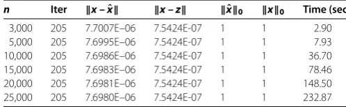
As indicated in Table , the ETA algorithm behaves very robust because the average number of times of iteration is identically equal to ; the recovered errorx–xˆand residualx–zare basically similar. In addition, the sparsityxof the recovered
Table 1 ETA’s computational results on LCPs withZ-matrices.
n Iter x –xˆ x – z ˆx0 x0 Time (sec.)
3,000 205 7.7007E–06 7.5424E-07 1 1 2.90
5,000 205 7.6995E–06 7.5424E-07 1 1 7.93
10,000 205 7.6986E–06 7.5424E-07 1 1 36.70
15,000 205 7.6983E–06 7.5424E-07 1 1 78.46
20,000 205 7.6981E–06 7.5424E-07 1 1 148.50
25,000 205 7.6980E–06 7.5424E-07 1 1 232.87
Table 2 SSG’s computational results on LCPs withZ-matrices.
n Iter x –xˆ ˆx0 x0 Time (sec.)
100 1,012 1.86E–05 1 1 2.46
200 972 1.70E–05 1 1 5.11
500 118 2.67E–06 1 1 3.88
1,000 118 1.58E–06 1 1 23.04
2,000 117 1.05E–06 1 1 139.15
3,000 117 8.69E–07 1 1 401.33
5,000 - - -
-ETA algorithm is exceptionally fast, which results in only . seconds being needed to address the problem with dimensionn= ,.
In order to illustrate the effectiveness of the ETA algorithm we proposed, we introduce another method of tackling the LCPs. In [], the authors established anlp( <p< ) reg-ularized minimization model:
min x∈Rnf(x) :=
FB(x)
+λxpp ()
and designed a sequential smoothing gradient (SSG) method to solve thelp regularized model and get a sparse solution ofLCP(q,M). The results are displayed in Table .
It can be discerned in Table , where ‘- -’ denotes the method is invalid. Although the sparsityxof the recovered solution is in all cases as large as and the recovered errors
x–xˆare pretty small, the average cpu time dramatically ascends with the matrix dimen-sionn, which manifests that SSG method for LCPs is appropriate for the small dimensional data set and thus SSG will not be appealing whennis relatively large. Contrasted with the SSG method, the ETA algorithm is more outstanding in the cpu time and the size of the solvable problems.
4.2 Test for LCPs with positive semidefinite matrices
In this subsection, we test ETA for randomly created LCPs with positive semidefinite matrices. First, we state the way of constructing LCPs and their solutions. Let a matrix Z∈Rn×r(r<n) be generated with the standard normal distribution andM=ZZ. Let the sparse vectorxˆbe produced by choosing randomly thes= .∗nnonzero components whose values are also randomly generated from a standard normal distribution. After the matrixMand the sparse vectorxˆhave been generated, a vectorq∈Rncan be constructed such thatxˆis a solution of theLCP(q,M). Thenxˆcan be regarded as a sparse solution of theLCP(q,M). Namely,
ˆ
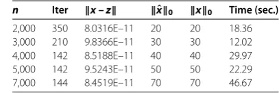
[image:10.595.166.423.209.296.2]Table 3 Results on randomly created LCPs with positive semidefinite matrices.
n Iter x – z ˆx0 x0 Time (sec.)
2,000 350 8.0316E–11 20 20 18.36
3,000 210 9.8366E–11 30 30 12.02
4,000 142 8.5188E–11 40 40 29.97
5,000 142 9.5243E–11 50 50 22.29
7,000 144 8.4519E–11 70 70 46.67
To be more specific, if xiˆ > then choose qi = –(Mxˆ)i, if xiˆ = then choose qi =
|(Mxˆ)i|– (Mxˆ)i. LetMand q be the input to our ETA algorithm and takez=e, c= max(svd(M)), λ= ., β = c, τ = ., γ = ., μ= /c, = e– , nmax= ,, K=max(, floor(,/n)). Then ETA will output a solutionx. Similarly, the residual
x–xˆ, average cpu time (in seconds), the average number of iteration times, and the residualx–zwill also be taken into consideration on valuating our ETA algorithm.
As manifested in Table , the ETA algorithm performs quite efficiently. Furthermore, the sparsityxof recovered solutionxis in all cases equal to the sparsityˆx, which means
the recover is exact. Likewise, the ETA algorithm is exceptionally fast in this example, which makes that only . seconds are needed to pursue the sparse solution of LCP when the dimensionn= ,.
4.3 Test for co-coercive nonlinear complementarity problem
We now consider a co-coercive nonlinear complementarity problems (NCP) with
F(x) =D(x) +Mx+q, ()
whereD(x) andMx+qare the nonlinear part and the linear part ofF(x), respectively. We formF(x) similarly as in [, ]. The matrixM=AA+B, whereAis ann×nmatrix whose entries are randomly generated in the interval (–, ), and a skew-symmetric matrix Bis generated in the same way. InD(x), the nonlinear part ofF(x), the components are
Dj(x) =aj∗arctan(xj)
andajis a random variable in (–, ). Then the sequent part of generating the sparse vector
ˆ
xand vectorq∈Rnsuch that
ˆ
x≥, F(xˆ)≥, xˆF(xˆ) = , and ˆx= .∗n
is similar to the procedure of Section .. LetMandqbe the input to our ETA algorithm and takez=e,c= ∗log(n),λ
= .,β = c,τ = .,γ = .,μ= /c, = e– ,
nmax= ,,K=max(, floor(,/n)), anda= –rand(n, ). Then ETA will output a
solutionx. Similarly, the average number of iteration times, the average residualx–z, the average sparsityxofx, and the average cpu time (in seconds) will also be taken into
consideration on valuating our ETA algorithm.
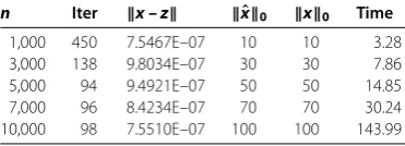
It is not difficult to see from Table that the ETA algorithm also performs quite effi-ciently in such nonlinear complementarity problems. The sparsityxof the recovered
solutionxare all equal to the sparsityˆx, that is, the recover is exact. What is also
Table 4 Results on co-coercive nonlinear complementarity problems.
n Iter x – z ˆx0 x0 Time
1,000 450 7.5467E–07 10 10 3.28
3,000 138 9.8034E–07 30 30 7.86
5,000 94 9.4921E–07 50 50 14.85
7,000 96 8.4234E–07 70 70 30.24
10,000 98 7.5510E–07 100 100 143.99
5 Conclusions
In this paper, we concentrate on finding sparse solutions of co-coercive nonlinear com-plementarity problems (NCPs). Anregularized projection minimization model is
pro-posed for relaxation, and an extragradient thresholding algorithm (ETA) is then designed for this regularized model. Furthermore, we analyze the convergence of this algorithm and show any cluster point of the sequence generated by ETA is a solution of NCP. Preliminary numerical results indicate that theregularized model as well as the ETA are promising
to find sparse solutions of NCPs.
Competing interests
The authors declare that they have no competing interests.
Authors’ contributions
All authors completed this paper together. All authors read and approved the final manuscript.
Author details
1Department of Applied Mathematics, Beijing Jiaotong University, Beijing, 100044, P.R. China.2Department of
Mathematics, Shijiazhuang University, Shijiazhuang, 050035, P.R. China. 3School of Mathematics, University of Southampton, Southampton, SO17 1BJ, UK.
Acknowledgements
We would like to thank the two referees for their valuable comments. This research was supported by the National Natural Science Foundation of China (71271021, 11001011, 11431002), the Fundamental Research Funds for the Central Universities of China (2013JBZ005) and the Scientific Research Fund of Hebei Provincial Education Department (No. QN20132030).
Received: 28 September 2014 Accepted: 6 January 2015
References
1. Cottle, RW, Pang, JS, Stone, RE: The Linear Complementarity Problem. Academic Press, Boston (1992)
2. Facchinei, F, Pang, JS: Finite-Dimensional Variational Inequalities and Complementarity Problems. Springer Series in Operations Research, vols. I and II. Springer, New York (2003)
3. Ferris, MC, Mangasarian, OL, Pang, JS: Complementarity: Applications, Algorithms and Extensions. Kluwer Academic, Dordrecht (2001)
4. Xie, J, He, S, Zhang, S: Randomized portfolio selection with constraints. Pac. J. Optim.4, 87-112 (2008)
5. Shang, M, Zhang, C, Xiu, N: Minimal zero norm solutions of linear complementarity problems. J. Optim. Theory Appl.
163, 795-814 (2014)
6. Candès, EJ, Randall, PA: Highly robust error correction by convex programming. IEEE Trans. Inf. Theory54, 2829-2840 (2006)
7. Candès, EJ, Recht, B: Exact matrix completion via convex optimization. Found. Comput. Math.9, 717-772 (2008) 8. Candès, EJ, Romberg, J, Tao, T: Stable signal recovery from incomplete and inaccurate measurements. Commun. Pure
Appl. Math.59, 1207-1223 (2006)
9. Donoho, DL: Compressed sensing. IEEE Trans. Inf. Theory52, 1289-1306 (2006)
10. Fukushima, M, Pang, JS: Some feasibility issues in mathematical programs with equilibrium constraints. SIAM J. Optim.8, 673-681 (1998)
11. Fukushima, M, Tseng, P: An implementable active-set algorithm for computing aB-stationary point of a mathematical program with linear complementarity constraints. SIAM J. Optim.12, 724-739 (2002)
12. Lin, G, Fukushima, M: New reformulations for stochastic nonlinear complementarity problems. Optim. Methods Softw.21, 551-564 (2006)
13. Luo, ZQ, Pang, JS, Ralph, D: Mathematical Programs with Equilibrium Constraints. Cambridge University Press, Cambridge (1996)
14. Figueiredo, MAT, Nowak, RD: An EM algorithm for wavelet-based image restoration. IEEE Trans. Image Process.12, 906-916 (2003)
15. Starck, JL, Donoho, DL, Candès, EJ: Astronomical image representation by the curevelet transform. Astron. Astrophys.
16. Daubechies, I, Defrise, M, De Mol, C: An iterative thresholding algorithm for linear inverse problems with a sparsity constraint. Commun. Pure Appl. Math.57, 1413-1457 (2004)
17. Figueiredo, MAT, Nowak, RD, Wright, SJ: Gradient projection for sparse reconstruction: application to compressed sensing and other inverse problems. IEEE J. Sel. Top. Signal Process.1, 586-597 (2007)
18. Zhu, T, Yu, ZG: A simple proof for some important properties of the projection mappings. Math. Inequal. Appl.7, 453-456 (2004)
19. Zhu, DL, Marcotte, P: Co-coercivity and its role in the convergence of iterative schemes for solving variational inequalities. SIAM J. Optim.6, 714-726 (1996)
20. Hale, ET, Yin, W, Zhang, Y: Fixed-point continuation for1minimization: methodology and convergence. SIAM J. Optim.19, 1107-1130 (2008)
21. He, BS, Liao, LZ: Improvements of some projection methods for monotone nonlinear variational inequalities. J. Optim. Theory Appl.112(1), 111-128 (2002)