2018 3rd International Conference on Computational Modeling, Simulation and Applied Mathematics (CMSAM 2018) ISBN: 978-1-60595-035-8
Statistical Analysis of Questionnaire Data via Cumulative Logistic
Regression Model
Xiao-na SHENG
1, Long LIU
2and Yu-qiu MA
1,*1
School of Information Engineering, Harbin University, Harbin 150086, China
2
School of Mathematical Sciences, Heilongjiang University, Harbin, 150080, China
*Corresponding author
Keywords: Cumulative logistic model, Rank variable, SAS.
Abstract. Based on a real questionnaire data, we build a cumulative logistic model to deal with the mutual relationship of the variables in the data. Aiming at the problem of too much designed variables, we apply statistical method to select those important ones and delete the useless ones without losing too much information. We also provide the analysis results for the data by the software SAS, and give some suggestions for the design of questionnaire. Our analysis also shows that the model built in paper can fit the questionnaire data very well, and it has higher preciseness rate of forecasting.
Introduction
With the incessant development of statistics, the method of logistic regression analysis attracts more and more attention [1,2]. However, as an important component part of logistic regression, the cumulative logistic regression is fairly less concerned in factual researches [3,4]. In 2013, to achieve the optimization configuration of human resource, a questionnaire about the service conduct situation of higher leaders in some direct-units of Heilongjiang province was carried out. Because too much problems and trivial content are designed in the questionnaire, it will bring bigger error if the usual method is used to analyze the data [5]. In this paper, the cumulative logistic regression is employed to integrate and analyze the data, which reduces some unnecessary variables. Then we use the model we built to perform some statistical forecasting, and the results are satisfactory.
There are 7 direct-units concerned in the survey, and 20675 questionnaires were sent out and collected. Two parts of content are designed: a. personal information of attendee; b. detail items on the service conduct situation, where 28 problems are included. Attendees can answer each problems based the factual situations of testing object (Rank: A, B, C, D). For the convenience of studying, we use variables xi (i=1,…,28) to denote the scores to the 28 questions, with values 1, 2, 3 and 4, where
variables xi (i=1,…,27) are the specific evaluations on the service conduct to a testing object, and
variable x28 is an integrative evaluation to the testing object.
Method
Cumulative Logistic Regression Model
Let the response variable y has J classes, i.e., y is an ordinal variable, and x={x1 ,..., xm} are
independent variables. Model
1
ln( ) , 1, 2, , 1,
1
m j
j k k k j
p
x j J
p
is called cumulative logistic regression model [3], where
1
( ) ( ) 1, 2, , 1
j j
i
p p y j x p y i x j J
are cumulative logistic functions, j (j1, 2,...,J1) are the latent thresholds of each class
ofy,k (k1, 2,...,m) are coefficients of model. Pretreatment for the Data
Search for the invalid questionnaires including blank ones and those whose answers are all 1, all 2, all 3, or all 4, then delete them [5,6]. The attendees who handed in the invalid questionnaires are irresponsible, and those corresponding data is useless to our analysis.
Model Building
Because the testing objects come from 7 different units, to diminish its impact on modeling, we combine the sample data from different units and model based on the integrated data.
Moreover, all variables concerned in the questionnaire are rank variables (4 ranks), and the variable about integrative evaluation also has 4 ranks, therefore, we consider building a cumulative logistic regression model [7-9]. We consider x28 to be dependent variable, and x={x1 ,..., x27} to be
independent variables. The corresponding cumulative logistic regression model is as follows:
27 28
1 28
( )
ln[ ] , 1, 2,3.
1 ( ) j k k k
p x j x
x j p x j x
The cumulative probability
27 1 27
1
28
( ) , 1, 2,3, 4;
1
j k k k
x j k k
k
x
j
e
p p x j x j
e
28
( | ), ( 1, 2,3, 4)
P x j x j denotes the probability that the integrative evaluation is A, B, C and D,
respectively; j is the integration ofj and ; j (j1, 2, ,J1) denotes the jth threshold,
where12 J1; k are the model coefficients.
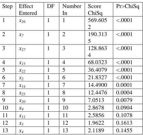
[image:2.595.177.421.543.774.2]There are totally 27 independent variables, however, we should introduce those with larger effects on the dependent variable, which will simply the analysis of data. In the paper, based on the statistical analysis software SAS [10,11], we use the method of forward selection to select the independent variables at a certain level, and 13 variables are finally retained in the model (see Table 1), i.e., variables x2, x4, x5, x7, x9, x11, x14, x15, x20, x22, x25, x26, x27.
Table 1. Output of forward variable selection by SAS.
Step Effect Entered
DF Number In
Score ChiSq
Pr>ChiSq
1 x26 1 1 569.605
2
<.0001
2 x7 1 2 190.313
5
<.0001
3 x27 1 3 128.863
4
<.0001
4 x15 1 4 68.0323 <.0001
5 x22 1 5 36.4079 <.0001
6 x2 1 6 21.8327 <.0001
7 x14 1 7 14.4900 0.0001
8 x25 1 8 12.4476 0.0004
9 x20 1 9 7.0513 0.0079
10 x9 1 10 2.8678 0.0904
11 x11 1 11 2.5856 0.1078
12 x5 1 12 1.9622 0.1613
Model Fit
We first consider whether the proportion hypothesis holds. If the hypothesis is declined, i.e., the regression lines of different cumulative log-odds are not parallel, the current cumulative logistic model will be not applicable. Otherwise, it will be applicable. The output results about the testing of the hypothesis by the SAS is presented in Table 2.
Table 2. Testing results of proportion hypothesis.
Chi-Square DF Pr>ChiSq
35.9836 12 0.0920
It can be seen from Table 2 that the value of statistic is 35.9836 (DF=12) with a p-value 0.092, so the test is not significant, i.e., the proportion hypothesis holds and the model we built is applicable. Besides, we also check the goodness of fit from aspects of deviance, Pearson 2 and R-Square, and the corresponding results are listed in Table 3.
Table 3. Testing results of goodness of fit.
Criterion Value DF Value/DF Pr>ChiSq
Deviance 649.2196 171
8
0.3779 1.0000
Pearson 170285.856 171
8
99.1187 <.0001
R-Square 0.7678 Max-rescaled R-Square 0.8618
[image:3.595.75.522.458.506.2]We find in Table 3 that the deviance test is not significant (p=1), the Pearson test is significant (p<0.0001), so the fit of model is good. At the same time, R-Square =0.7678, which means that the integrative evaluation variable has strong persuasion in the model. To give reasonable explains of the considered cumulative logistic model, we also provide the corresponding results of likelihood ratio (LR) test and Wald test (see Table 4).
Table 4. 2 and Wald test results for the data.
Test Chi-Square DF Pr>ChiSq
LR 1410.6027 13 <.0001
Wald 4 11.5647 13 <.0001
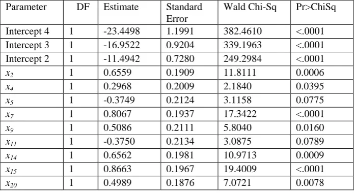
[image:3.595.124.473.604.794.2]Table 4 shows that the value of LR statistic is 1410.6027 with a small p-value, so the selected independent variables have significant explainable ability. Moreover, the value of Wald statistic is 411.5647 also with a small p-value, which means that the regression coefficients are significant. All the results from Tables 2 to 4 show that the model we built has good fit to the questionnaire data. The final results of regression analysis are listed in Table 5.
Table 5. Logistic regression analysis for integrative evaluation to independent variables.
Parameter DF Estimate Standard Error
Wald Chi-Sq Pr>ChiSq
Intercept 4 1 -23.4498 1.1991 382.4610 <.0001
Intercept 3 1 -16.9522 0.9204 339.1963 <.0001
Intercept 2 1 -11.4942 0.7280 249.2984 <.0001
x2 1 0.6559 0.1909 11.8111 0.0006
x4 1 0.2968 0.2009 2.1840 0.0395
x5 1 -0.3749 0.2124 3.1158 0.0775
x7 1 0.8067 0.1937 17.3422 <.0001
x9 1 0.5086 0.2111 5.8040 0.0160
x11 1 -0.3750 0.2134 3.0875 0.0789
x14 1 0.6562 0.1981 10.9713 0.0009
x15 1 0.8663 0.1967 19.4009 <.0001
x22 1 0.7374 0.1689 19.0620 <.0001
x25 1 0.6519 0.1816 12.8789 0.0003
x26 1 0.3630 0.2015 3.2448 0.0716
x27 1 1.5108 0.1949 60.060 <.0001
From Table 5 we can see that all the variablesx2, x4, x5, x7, x9, x11, x14, x15, x20, x22, x25, x26 and x27
have significant impact to the integrative evaluation. By the practical study on the problem background, we also find that the selection of these variables is exactly reasonable. So we suggest that only retaining the 13 variables in later questionnaire is enough. Combined with the above analysis indexes, the model we built based on the questionnaire data is as follows:
1
2 4 5 7 9 11 14 15 20 22 25 26 27
2 3 4
1 2
2 4 5 7
3 4
ln( ) 23.449 0.656 0.297 0.375 0.807 0.509 0.375 0.656 0.866 0.499 0.737 0.652 0.363 6 1.511 , (1)
ln( ) 16.952 0.656 0.297 0.375 0.807 0.5
p
x x x x x x x x x x x x x
p p p p p
x x x x
p p
9 11 14 15 20 22 25 26 27
1 2 3
2 4 5 7 9 11 14 15 20 22
4
09 0.375 0.656 0.866 0.499 0.737 0.652 0.363 6 1.511 , (2)
ln( ) 11.494 0.656 0.297 0.375 0.807 0.509 0.375 0.656 0.866 0.499 0.737 0
x x x x x x x x x
p p p
x x x x x x x x x x
p
25 26 27
.652x 0.363x 6 1.511 x . (3)
After further checking and validation, the preciseness rate of forecasting by the model we built can attain 86.75%, which is very ideal in practice.
Factor Analysis for Affecting Integrative Evaluation
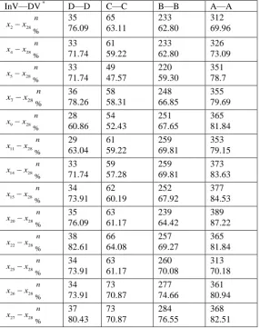
[image:4.595.156.443.426.788.2]To further make clear the mutual relationships between the dependent variable and each independent variable, we also consider factor analysis, from which we can directly see the contribution of each independent variable to the dependent variable. The analysis results of consistency for the variables are presented in Table 6.
Table 6. Contingency table for consistency of variables.
InV—DV * D—D C—C B—B A—A
2 28
%
n
x x 35 76.09 65 63.11 233 62.80 312 69.96
4 28
%
n
x x 33
71.74 61 59.22 233 62.80 326 73.09 5 28 % n
x x 33
71.74 49 47.57 220 59.30 351 78.7 7 28 % n
x x 36
78.26 58 58.31 248 66.85 355 79.69 9 28 % n
x x 28
60.86 54 52.43 251 67.65 365 81.84 11 28 % n
x x 29
63.04 61 59.22 259 69.81 353 79.15 14 28 % n
x x 33
71.74 59 57.28 259 69.81 373 83.63 15 28 % n
x x 34
73.91 62 60.19 252 67.92 377 84.53 20 28 % n
x x 35
76.09 63 61.17 239 64.42 389 87.22 22 28 % n
x x 38
82.61 66 64.08 257 69.27 365 81.84 25 28 % n
x x 34
73.91 63 61.17 260 70.08 313 70.18 26 28 % n
x x 34
73.91 73 70.87 277 74.66 361 80.94 27 28 % n
x x 37
80.43 73 70.87 284 76.55 368 82.51
Table 6 shows that the rank selection of x28 has higher consistency with that of each independent
variable. When the rank selections between them are not consistent, the evaluation of independent variable usually has higher rank than that of dependent variable, which shows that the attitude of attendee is careful. In the consistency results, we can see that variables x2, x4, x5 and x25 each has a
consistency rate about 67% with x28; and the consistency rate between variables x7, x9, x11, and x28 is
about 78%, which shows that protecting week-population is taken as a fundamental rule when the attendees fill in the questionnaire.
Conclusion
In this paper, we analyze a questionnaire data by building a cumulative logistic model, which deals with the problem of the too much designed problems, and therefore simplifies the content of questionnaire. Of course, the completeness of data is retained to a large degree[3], and the preciseness of analysis can also be guaranteed.
From the evaluation results to the testing objects, we find that people more care those aspects associated with their work and life, and the execution status to the necessary rules is a focus of people’s attention. All in all, the first task of service conduct situation is to begin from the people’s livelihood, and only those rules which can be executed authentically in practice are good ones. In fact, there are still problems that are worthy studying further in the questionnaire data. For example, how to deal with the absence problem of some variables, how to compare the scores of each testing object in the same unit [12], and so on. We will go on carrying out our study in future work.
Acknowledgement
This paper is supported by the 3rd National Agricultural Census Leading Group Project of Heilongjiang Provincial Government (no.028).
References
[1]M. Juan, W. Philippe, G. Nermin, et al., An Original Stepwise Multilevel Logistic Regression Analysis of Discriminatory Accuracy: The Case of Neighbourhoods and Health. Plos One, 11(2016): e0153778.
[2]M. C. Simmonds, J. P.Higgins, A general framework for the use of logistic regression models in meta-analysis. Statistical Methods in Medical Research, 25(2016): 2858.
[3]M. H. Joseph. Logistic Regression Models, Chapman & Hall/CRC Press, 2009.
[4]L. F. Huntsinger, N. M. Rouphail, P. Bloomfield, Trip Generation Models Using Cumulative Logistic Regression. Journal of Urban Planning & Development, 139(2013): 176-184.
[5]J. Rattray, Essential elements of questionnaire design and development. Journal of Clinical Nursing, 16(2007): 234-243.
[6]Y.Song, Y. Son, D. Oh, Methodological Issues in Questionnaire Design. Journal of Korean Academy of Nursing, 45(2015): 323-328.
[7]A. Agresti, Analysis of Ordinal Categorical Data. New York: Wiley, 1984.
[8]S. L. Newman, R. Tumin, R. Andridge, et al. Family Meal Frequency and Association with Household Food Availability in United States Multi-Person Households: National Health and Nutrition Examination Survey 2007-2010. Plos One, 10(2015):e0144330.
[10]M. E. Stokes, C. S. Davis, G. G. Koch, Categorical Data Analysis Using the SAS System (2nd Edition). SAS Institute and Weily, 2003.
[11]Mervyn G. Marasinghe, William J. Kennedy. SAS for Data Analysis, New York: Springer– Verlag, 2008.