An alternating linearization bundle method for a class of nonconvex nonsmooth optimization problems

R E S E A R C H

Open Access

An alternating linearization bundle

method for a class of nonconvex nonsmooth

optimization problems

Chunming Tang

1

_{, Jinman Lv}

1

_{and Jinbao Jian}

2*

*_{Correspondence:}

[email protected]

2_{College of Science, Guangxi}

University of Nationalities, Nanning, P.R. China

Full list of author information is available at the end of the article

Abstract

In this paper, we propose an alternating linearization bundle method for minimizing the sum of a nonconvex function and a convex function, both of which are not necessarily differentiable. The nonconvex function is first locally “convexified” by imposing a quadratic term, and then a cutting-planes model of the local

convexification function is generated. The convex function is assumed to be “simple” in the sense that finding its proximal-like point is relatively easy. At each iteration, the method solves two subproblems in which the functions are alternately represented by the linearizations of the cutting-planes model and the convex objective function. It is proved that the sequence of iteration points converges to a stationary point. Numerical results show the good performance of the method.

Keywords: Bundle method; Alternating linearization; Local convexification; Global convergence

1 Introduction

In this paper, we consider the structured nonconvex minimization problem

min

x∈Rn

F(x) :=f(x) +h(x), (1)

wheref :Rn_{→Ris possibly a nonconvex nonsmooth function andh:R}n_{→(–∞,∞] is} a closed proper convex function.

Problems of the form (1) often appear in practice, such as signal processing, image re-construction, engineering, optimal control, and so on. Three typical examples are given below.

Example1 (Unconstrained transformation of a constrained problem) Consider the con-strained problem

minf(x) :x∈C, (2)

where f is possibly a nonsmooth nonconvex function andC is a convex subset ofRn_. Problem (2) can be written equivalently as

min

x∈Rnf(x) +ıC(x), (3)

whereıC is the indicator function ofC, i.e.,ıC(x) equals 0 onCand infinity elsewhere. Clearly, problem (3) is a special case of problem (1) withh(x) =ıC(x). We note that the proximal point ofıCcan easily be calculated or even has a closed-form solution ifChas some special structure.

Example2 (Nonconvex regularization of a convex function) Consider thelq(0 <q< 1) regularization problem

min

x∈Rn 1

2Ax–b 2_+λx

q, (4)

which has many practical applications in compressed sensing and imaging science (see e.g., [1]), wherexq= (

n

i=1|xi|q)1/q. The objective function of problem (4) is also the sum of a convex function and a nonconvex function.

Example3 (Convex regularization of a nonconvex function) Hare et al. [2] studied the function of the form

F(x) = n

i=1 fi(x)+

1 2x

2_{, (5)}

wherefi(x) :Rn_{→R,i= 1, . . . ,nare Ferrier polynomials defined as}

fi(x) =ix2_i – 2xi+ n

j=1 xj.

It is well known thatf(x) =n_i=1|fi(x)|is a nonconvex nonsmooth function, andh(x) = 1

2x

2_{is a simple convex function.}

In this paper, we consider to minimize the sum of a nonconvex function and a convex function with the form of (1). In particular, we assume thatf is lower-C2 _andhis “sim-ple” in the sense that minimizinghplus a quadratic term is relatively easy. The method presented in this paper can be viewed as a generalized version of the methods given in [9] and [13]. On one hand, we generalize the method of [9] from minimizing the sum of two convex functions to the sum of a nonconvex function and a convex function. On the other hand, we generalize the method of [13] from minimizing a single nonconvex nonsmooth function to the sum of two functions.

Our method will produce three sequences of points:{z_{}, {y}and{x}k()_{}, where{z}}

is the sequence of proximal points,{y_{}is the sequence of trial points, and{x}k()_{}is the} sequence of stability centers (i.e.,xk()_{∈ {y}is the “best” point obtained so far for iteration} , which will be abbreviated asxkif there is no confusion). More precisely, our method will alternately solve the following two subproblems:

z+1_{:=arg min ϕˇ (·) +h}¯

–1(·) +

1

2μ·–x k2

, (6)

y+1:=arg min ϕ¯ (·) +h(·) +1

2μ·–x k2

, (7)

whereϕˇ is a cutting-planes model [14, 15] of the local convexification function off at iteration, which is based on the idea of the redistributed proximal bundle method in [13] and will be made more precise later;h¯–1is a linearization ofhat iteration– 1;ϕ¯ is a linearization ofϕˇ ;μis the proximal parameter. Our convergence analysis shows that, under suitable assumptions, any accumulation point of the sequence{xk_{}is a stationary} point ofFif there is an infinite number of serious steps; otherwise, the last stability center is a stationary point ofF.

This paper is organized as follows. In Sect. 2, we review some basic definitions and re-sults required for this work. In Sect. 3, we present the alternating linearization bundle method for problem (1). Section 4 examines the convergence properties of the algorithm. Some preliminary numerical results are given in Sect. 5. The Euclidean inner product in

Rn_{is denoted byx,y=x}T_{y, and the associated norm by · .}

2 Preliminaries

In this section, we recall some basic definitions and results that are closely relevant to our method, which can be found in [13, 16, 17].

– Thelimiting subdifferentialoff atx¯is defined by

∂f(x) :=¯ lim

x→¯x_f(x)sup_→f(x)¯ ∂ˆf(x),

where∂ˆf(x)¯ is theregular subdifferentialdefined by

ˆ

∂f(x) :=¯ g∈Rn:lim

x→¯xinfx=x¯

f(x) –f(x) –¯ g,x–x¯ x–x¯ ≥0

.

– The functionf isprox-boundedif there existsR≥0such that the function

f(·) +1₂R · 2_{is bounded below. The corresponding threshold is the smallestrpb≥0}

such thatf(·) +1₂R · 2is bounded below for allR>rpb.

– The functionf islower-C2_{on an open setVif for eachx¯∈V there is a neighborhood} Vofx¯upon which a representationf(x) =max_t∈Tft(x)holds, whereT is a compact

set and the functionsftare of classC2onVsuch thatft,ft and2ftdepend continuously on(t,x)∈T×V.

– Theproximal point mappingof the functionf at the pointx∈Rn_{is defined by}

pRf(x) :=arg min ω∈Rn f(ω) +

1

2Rω–x 2

.

Lemma 1([16]) Suppose that the function f is lower-C2_{on V andx¯∈V.Then there exist}

ε> 0,K> 0,andρ> 0such that

(i) for any pointx0and parameterR≥ρthe functionf+1₂R ·–x02is convex and finite valued on the closed ballB¯ε(x)¯ ,and

(ii) the functionf is Lipschitz continuous with constantKonB¯ε(x)¯ .

Theorem 1([16]) Suppose that the lower semicontinuous function f is prox-bounded with threshold rpband lower-C2 _{on V.Letx¯∈V and letε> 0,K> 0andρ> 0be given by} Lemma 1.Then x is a stationary point of f if and only if¯ x¯=pRf(x)¯ for any R>Rx¯ :=

max{4K/ε,ρ,rpb}.

Assumption 1([13]) Givenx0∈RnandM0≥0, there exist an open bounded setOand a functionHsuch thatL0:={x∈Rn_:f(x)≤f(x0_{) +M0} ⊂O, andHis lower-C}2_onOwith H≡f onL0.

Theorem 2([13]) For a function f satisfying Assumption1,the following results hold:

(i) The level setL0is nonempty and compact.

(ii) There existsρid_{> 0such that,for anyρ≥ρ}id_{and any giveny∈L0,the function} f +1

2ρ ·–y

2_{is convex onL0.}

(iii) The functionf is Lipschitz continuous onL0.

3 The alternating linearization bundle method

3.1 Motivation and framework

The classic proximal point algorithm (see e.g. [18]) for solving problem (1) generates the new iterate by

y+1_{=arg min f(·) +h(·) +}1 2R·–y

2

, (8)

whereR> 0 is the proximal parameter.

However, sincef is a nonconvex function, solving problem (8) may not be easy and is usually as difficult as the original problem (1). Therefore, we will tackle the difficulty via the following three steps.

ηandμ which are nonnegative and satisfyR=η+μ. Then the problem (8) (after

replacingy_byxk_{) can be written as}

y+1=arg min ϕ(·) +h(·) +1

2μ·–x k2

, (9)

where

ϕ(·) =f(·) +

1 2η·–x

k2

(10)

is called the local convexification function of f, since it is convex wheneverη is large enough (see Theorem 2).

2.Generate the cutting-planes model of ϕ. Letbe the current iteration index,yi_,i∈ J⊆ {0, 1, . . . ,}be trial points generated in the previous iterations, andg_fi∈∂f(yi). Define

the cutting-planes model ofϕby

ˇ

ϕ(·) =max

i∈J

fyi+1 2ηy

i_–xk2

+g_fi+η

yi–xk,·–yi, (11)

whereg_fi=gf(yi)∈∂f(yi). Therefore, we obtain an approximate version of problem (9) as follows:

y+1_{:=arg min ϕˇ (·) +h(·) +}1

2μ·–x k2

. (12)

3.Apply the alternating linearization bundle strategy to solve problem(12). Since prob-lem (12) may still be difficult, motivating by the idea of the alternating linearization bun-dle [9], we consider to alternately solve the following two subproblems:

z+1:=arg min ϕˇ (·) +h¯–1(·) +

1

2μ·–x k2

, (13)

y+1_{:=arg min ϕ¯ (·) +h(·) +}1

2μ·–x k2

. (14)

The above two subproblems are much easier to solve, whose objective functions are alter-nately represented by linear models ofh(·) andϕˇ (·), respectively.

3.2 Further description via bundle terminologies

Bundle methods [19–21] are among the most robust and reliable methods to solve gen-eral nonsmooth optimization problems, which can be considered stabilized variants of cutting-planes method [14, 15]. In general, for a convex functionh, bundle methods store the trial pointsyi,i∈Jwith their function values and subgradients in a bundle of

infor-mation:

i∈J

and a pointxk_:=xk() _{(calledstability center) which is the “best” point obtained so far.} A storage-saving form of (15) (refer to the current stability centerxk_{) is given by}

i∈J

ei,k_h ,g_hi∈∂

ei_h,kh

xk,

where ∂ehis thee-subdifferential ofhin convex analysis, and ei,kh are the linearization errors ofhdefined by

ei,k_h =hxk_–hyi_+gi h,xk–yi

. (16)

Following the notations above, the bundle information of the functionϕ(·) can be writ-ten as (see also [13]):

i∈J

ei,k_f ,dk_i,k_i,g_fi with ⎧ ⎪ ⎪ ⎪ ⎪ ⎪ ⎨ ⎪ ⎪ ⎪ ⎪ ⎪ ⎩

ei,k_f =f(xk_{) – (f(y}i_{) +g}i

f,xk–yi), dk_i =1₂yi_–xk2_,

gi

f ∈∂f(yi),

k_i =yi–xk,

(17)

whereei,k_f anddk

i are the linearization errors off and12 ·–xk2, respectively,gfiis a sub-gradient off atyi, andk_i is the gradient of 1

2 ·–x

k2_atyi_{. From (17), we know thate}i,k f , d_ikandk_i depend on the pointxk_{, so they should be updated whenever a new stability} center is generated (details are given below).

By the optimality conditions of subproblem (13), there exists a multiplier vector (α_i,i∈ J)∈Ssuch that

z+1=xk– 1

μ

i∈J

α_ig_fi+ηk_i+g_h–1

, (18)

whereS_{denotes the unit simplex inR}|J|_andg–1

h =∇ ¯h–1(z+1).

As iterations go along, the number of elements in the bundle may increase infinitely, which could lead to serious problems with storage and computation. The subgradient ag-gregation strategy [22] is the most popular and efficient way to overcome such a difficulty. We use the notationg–

η to denote the aggregate subgradient, i.e.,

g– η :=

i∈J

α_ig_fi+ηk_i∈∂ϕˇ z+1_{. (19)}

Define the strongly active set of subgradients by

Jact:=

i∈J:α_i> 0

.

Then the corresponding aggregate bundle elements are given by

e–_f,d_–k,k–,g–

f

:=

i∈J

α_iei,k_f ,dk_i,k_i,g_fi=

j∈Jact

Therefore

gη–=

i∈J

α_ig_fi+ηki

=g_f–+ηk–=μ

xk–z+1–g_h–1.

Here, as in [13, 23], we use negative index –to express the aggregate bundle elements, henceJ⊆ {–, –+ 1, . . . , 0, 1, . . . ,– 1,}in general.

By making use of the notations above, the cutting-planes modelϕˇ in (11) can be rewrit-ten as:

ˇ

ϕ(·) =fxk+max

i∈J

–ei,k_f +ηdk_i+gi_f+ηk_i,·–xk. (21)

Note that, for allj∈Jact

we have

ˇ

ϕz+1=fxk–ej,k_f –ηd_jk+g_fj+ηk_j,z+1–xk, (22)

and the aggregate model ofϕˇ inJis

˜

ϕ–(·) =f

xk–e–_f,k–ηdk_–+

g_f–+ηk_–,·–xk.

For a new stability centerxk+1_{, the bundle elements can be updated by (see [13])}

ei,k+1_f =ei,k_f +fxk+1–fxk+g_fi,xk+1–xk,

d_ik+1=d_ik+1 2x

k+1_–xk2₊k

i,xk+1–xk

,

k+1_i =k_i +xk–xk+1.

(23)

On the other hand, sincefis possibly nonconvex, the linearization errorsei,k_f +ηd_ik,i∈J

may be negative, and therefore the modelϕˇ is not necessarily a lower approximation to

ϕ. In the case ofei,k_f +ηdk_i ≥0, one has

g_fi+ηk_i ∈∂_ei,k f +ηdkiϕˇ

xk. (24)

In order to ensure that the linearization errors are all nonnegative, the convexification parameterηshould be adjusted to asymptotically estimate the ideal convexity threshold

ρid_{in Theorem 2. Hare et al. [2] suggested a lower bound forηas follows:}

ηmin := max

i∈J,dik>0 –e

i,k f

dk_i , (25)

which guarantees thatei,k_f +ηdk_i ≥0 for alli∈Jwheneverη≥ηmin .

Finally, in our algorithm, we define the predicted descentδand the linearization error

εas follows:

δ:=fxk+1 2ηy

ε:=Fxk–ϕ¯xk+h¯

xk. (27)

For a fixed parameterκ∈(0, 1), adescent stepis taken if

Fy+1≤Fxk–κδ, (28)

holds, and then update the stability centerxk+1_=y+1_{. Otherwise, anull stepoccurs, and} then the aggregate linearization and the new linearization are used to produce a better modelϕˇ+1.

3.3 The algorithm

Algorithm 1

Step0. (Initialization). Select a starting pointy0_{and setx}0_=y0_{. Set parametersM> 0,} R0> 0,κ∈(0, 1),≥0, and≥1. Initialize the iteration counter= 0, the descent step counterk:=k() = 0 withi0= 0. Set (μ0,η0) = (R0, 0) andJ0:={0}. Computef(x0),gf0∈

∂f(x0_{) and the bundle information (e}0,0

f ,d00,00) := (0, 0, 0). Sets–1h =gh0∈∂h(x0). Step1. Findz+1_{by solving subproblem (13), and set}

¯

ϕ(·) =ϕˇ z+1_+s ϕ,·–z

+1 _{with s} ϕ=μ

xk–z+1_–s–1

h . (29)

Step2. Findy+1_{by solving subproblem (14), and set}

¯ h(·) =h

y+1_+s

h,·–y+1

with s

h=μ

xk–y+1_–s

ϕ. (30)

Step3. (Stopping criterion). Computef(y+1_),h(y+1_),g+1 f ∈∂f(y

+1_{) andg}+1 h ∈∂h(y

+1_). Ifδ≤, then STOP. Otherwise, compute the new bundle elements by

k₊₁:=y+1_–xk_{, d}k

+1:=k+1 2

/2,

e_f+1,k:=fxk–fy+1_+g+1 f ,k+1

.

Select a new index setJ+1satisfying

J+1⊇ {+ 1,ik} and ⎧ ⎨ ⎩

either J+1⊇Jact,

or J+1⊇ {–}.

(31)

Step4. (Descent test). If (28) holds, declare a descent step, setk(+ 1) =k+ 1,ik+1=

+ 1,xk+1_=y+1_{, and update the bundle elements by (23). Otherwise, declare a null step,} and setk(+ 1) =k().

Step5. (Updateη). Update the convexification parameter by ⎧

⎨ ⎩

η+1:=η ifηmin+1≤η,

η+1:=ηmin+1 and R+1:=μ+η+1 otherwise.

(32)

Step6. (Updateμ). IfF(y+1_{) >F(x}k_{) +M, then the objective increase is unacceptable,} letμ+1:=μand loop to Step 1; otherwise, setμ+1:=μ.

Remark1 (1) The predicted descentδand the linearization errorεare nonnegative (the details are given below); (2) in Step 6, ifF(y+1_{) >F(x}k_{) +Mholds, then the current model} is considered as “bad”, so we should become more “conservative”, and therefore increase the proximal parameterμby settingμ+1=μ. In the next section, we will prove that the number of increasingμis finite; (3) the parametersμ,ηin the algorithm will be stable eventually.

Lemma 2 The predicted descentδ and the linearization errorε are nonnegative,and

satisfy

ε=δ–R+μ 2μ2 s

2_{, with s=s} ϕ+s

h. (33)

Proof In Step 2, from (30) and (18) we knowg–1

h =sh–1, hence

g– η =μ

xk–z+1_–g–1 h =μ

xk–z+1_–s–1

h =sϕ. (34)

Next, we proveδ≥0 andε≥0. From (26) and (29) we have

δ=fxk+1 2ηy

+1_–xk2_+hxk_{–ϕ¯ y}+1_+h¯

y+1

=fxk+1 2ηy

+1_–xk2

+hxk–ϕˇ z+1_–s

ϕ,y+1–z+1

–hy+1

=fxk–ϕˇ z+1–sϕ,y

+1_–z+1₊1 2ηy

+1_–xk2_+hxk_–hy+1_{. (35)}

Letj= –in (22) and from (34) we can obtain

fxk–ϕˇ z+1–sϕ,y

+1_–z+1

=fxk–fxk–e–_f–ηdk_–+

g_f–+ηk_–,z+1–xk–sϕ,y

+1_–z+1

=e–_f+ηdk_––

sϕ,z

+1_–xk_–s ϕ,y

+1_–z+1

=e–_f+ηdk–+

sϕ,xk–y

+1_{. (36)}

On the other hand, from (30), we have

–hy+1= –hy+1–s_h,xk–y+1+s_h,xk–y+1

= –h¯

xk+s_h,xk–y+1. (37)

Hence, by combining (36), (37) and (30), (35) can be written as

δ=e–_f+ηdk_–+

sϕ,xk–y +1₊1

2ηy

+1_–xk2_+hxk_–h¯

xk

+s

h,xk–y+1

(38)

=e–_f+ηdk_–+

μxk–y+1,xk–y+1+1 2ηy

+1_–xk2

+hxk–h¯

xk

=e–_f+ηdk_–+

R+μ

2 y

+1_–xk2_+hxk_–h¯

In Step 5, the update forηis done to ensureη≥ηmin

for all iterations, so thate–f+ηdk–≥

0. Therefore, the predicted descentδ≥0 sincehis convex. Forε, from (27), one has

ε=Fxk–ϕ¯ xk+h¯

xk

=fxk+hxk–ϕˇ z+1–sϕ,xk–z +1_–h¯

xk

=fxk–ϕˇ z+1_–s ϕ,x

k_–z+1_+hxk_–h¯

xk. (40)

Similar to (36), we have

fxk–ϕˇ z+1–sϕ,xk–z +1

=fxk–fxk–e–_f–ηdk_–+

g_f–+ηk_–,z+1–xk

–sϕ,xk–z +1

=e–_f+ηdk_––

sϕ,z

+1_–xk_–s ϕ,xk–z

+1

=e–_f+ηdk–. (41)

Thus, we have

ε=e–f+ηd–k+h

xk–h¯

xk≥0. (42)

Equation (33) follows immediately from (39) and (42).

From (33), We know thatδ≥ε. Therefore, ifδ≤, thenε≤. So, we only useδ≤

as the termination criterion in Step 5.

Lemma 3 The vectors s ϕand s

hof(30)and(29)are in fact subgradients,i.e.,

sϕ∈∂ϕˇ

z+1 and s_h∈∂h

y+1. (43)

Furthermore,we have

¯

ϕ≤ ˇϕ and h¯≤h. (44)

Proof Letφ_fandφ_hdenote the objectives of (13) and (14), respectively, i.e.,

φ_f(·) :=ϕˇ(·) +h¯–1(·) + 1

2μ·–x k2

, (45)

φ_h(·) :=ϕ¯(·) +h(·) +1

2μ·–x

k2_{. (46)}

By (13), (29) and the optimality condition of (45), we have

which impliess

ϕ∈∂ϕˇ(z+1). Similarly, by (14) and the optimality condition of (46), we

obtain

0∈∂hy+1_+s ϕ+μ

xk–y+1_=∂hy+1_–s

h,

which impliess_h∈∂h(y+1). So (43) holds.

Equation (44) follows immediately from (43).

4 Convergence

In this section, we will study the convergence properties of Algorithm 1. Firstly, based on the objective function of problem (1), we need to slightly modify Assumption 1 as follows.

Assumption 2 Givenx0∈RnandM0≥0, there exist an open bounded setOand a func-tionHsuch thatL0:={x∈Rn_:F(x)≤F(x0_{) +M0} ⊂O, andH is lower-C}2_onOwith H≡f onL0.

For convenience, we assume that Assumption 2 holds throughout the rest of convergence analysis.

In addition, from [24] we know that, iff is a locally Lipschitz continuous function, then the subgradients off are locally bounded, i.e.,

g_fis bounded ifyis bounded. (47)

Further, as in [9], it follows that the model subgradientss

ϕin (43) satisfy

sϕ

is bounded ifyis bounded. (48)

Remark2 Note that (47) implies that{g

ϕ:=gf+ηi} (gϕ∈∂ϕˇ) is bounded if{y}is

bounded, since {

i} in (17) is bounded if {y

_{} is bounded. Sinces}

ϕ∈∂ϕˇ , then s ϕ ∈ conv{gϕj}j∈J, thus we haves

ϕ ≤maxj=1g j

ϕ, and the modelϕˇ satisfies condition (48)

automatically when (47) holds.

The following lemma shows the properties of the model functionϕˇ, whose proof can

be found in [13, 16].

Lemma 4 For the model functionϕˇ and convexification parameterη,we have

(i) ϕˇ is a convex function. (ii) Ifη≥ηmin,then

ˇ

ϕxk≤fxk. (49)

(iii) Ifη+1=η,and eitherJ+1⊇JactorJ+1⊇ {–},then

ˇ

ϕ+1(·)≥ ˇϕz+1+sϕ,·–z +1

(iv) IfJ⊇ {},then

ˇ

ϕ(·)≥fy+1 2ηy

–xk2+g_f+ηy–xk,·–y,

for someg

f ∈∂f(y

_).

(v) Ifη≥ρid,then

ˇ

ϕ(ω)≤f(ω) +

1

2ηω–x k2

for allω∈L0. (50)

From the updating rule in Step 5 of Algorithm 1, the convexification parameterηis either unchanged or increasing. The following lemma shows thatηcan be fixed in a finite number of iterations, whose proof can be found in [13].

Lemma 5 There exist an index1and a positive constantη> 0such that

η≡η, for all≥1.

Lemma 6 Suppose that there exists an integer K such that,for all≥K,only null steps occur without increasingμ.Then the following results hold:

(i) The sequences

φ_fz+1=ϕˇ

z+1+h¯–1

z+1+1 2μz

+1_–xk2

≥K ,

φ_hy+1=ϕ¯ y+1+hy+1+1 2μy

+1_–xk2

≥K

are nondecreasing and convergent.

(ii) The sequences{y+1_}and{z+1_{}are bounded,z}+1_–y+1 _→0and z+2_–y+1 _{→0as→ ∞.}

Proof First, using partial linearizations of the subproblems to show (i) is hold. Fixed≥K. By the definitions in (13) and (29), we haveϕ¯ (z+1_{) =ϕˇ (z}+1_{) and}

z+1=arg min φ¯_f(·) :=ϕ¯(·) +h¯–1(·) +

1

2μ·–x k2

, (51)

from∇ ¯φ_f(z+1_{) = 0. Sinceφ}¯

f is quadratic andφ¯

f(z

+1_{) =φ}

f(z

+1_{), by Taylor’s expansion}

¯

φ_f(·) =φ¯_fz+1+∇ ¯φ_fz+1·–z+1+1 2μ·–z

+12

=φ_fz+1+1 2μ·–z

+12_{. (52)}

Similarly, by the definitions in (14) and (30), we haveh¯(y+1) =h(y+1), and

y+1_{=arg min φ}¯

h(·) :=ϕ¯ (·) +h¯(·) +

1

2μ·–x k2

¯

φ_h(·) =φ_hy+1+1

2μ·–y

+12_{. (54)}

Next, to bound the objective values of the linearized subproblem (51) and (53) from above, we useϕ¯ ≤ ˇϕandh¯–1≤h,h¯≤hof (44) andϕˇ(xk)≤f(xk) in (ii) of Lemma 4

φ_fz+1+1 2μx

k_–z+12_=φ¯

f

xk≤ ˇϕxk+hxk≤Fxk, (55)

φ_hy+1₊1 2μx

k_–y+12

=φ¯_hxk≤ ˇϕxk+hxk≤Fxk. (56)

From (14) and (51), we haveφ¯_f≤φ_h. On the other hand, since only null step occurred, so xk+1_=xk_{, the algorithm ensures thatμ=μ}

+1, andϕ¯ ≤ ˇϕ+1by (iii) of Lemma 4, we can obtainφ¯

h≤φf+1. By (52) and (54), we see that

φ_fz+1₊1 2μy

+1_–z+12

=φ¯_fy+1_≤φ

h

y+1_{, (57)}

φ_hy+1+1 2μz

+2_–y+12

=φ¯_hz+2≤φ_f+1z+2. (58)

In particular, from (57) and (58), we have the relation

φ_fz+1_≤φ

h

y+1_≤φ+1 f

z+2

which implies that{φ_f(z+1_)}

≥Kand{φh(y+1)}≥Kare nondecreasing sequences. Together with the bound ofF(xk_{) from (55) and (56), the convergence is established.}

For (ii), we have proved the convergence of{φ

f(z+1)}and{φh(y+1)}in (i) when≥K, so there must have a common limit, sayφ∞≤F(xk), such that

φ_fz+1→φ∞, φ_hy+1→φ∞ (59)

and we havez+1_–y+1 _{→0 andz}+2_–y+1 _{→0 from (57) and (58),{y}+1_}and{z+1_} are bounded from (55) and (56). Then the sequences{g

f}and{s

ϕ}are bounded by (47)

and (48).

The following lemma shows that the number of times of increasingμis finite.

Lemma 7 Suppose that ik∈J,and let Nbe the number of times of increasingμ.Then

there exists a positive constant L such that

N≤

_ln L2

Mμ0

ln

, (60)

whereais the smallest integer greater than or equal to a.As a result,there exists an index

2such that

Proof Letrbe the index corresponding to therth time thatμincreases, then whenr+ 1≤<r+1, we have

μ=rμ0. (61)

Sinceik∈J, from (24), we obtain gik ∈∂ϕˇ(xk) by writingi=ik, and it also holds that

g_fik∈∂f(xk_{) from (21), sog}ik

f is bounded. Hence

pμ(ϕ¯ +h)

xk

=arg min ϕ¯ (y) +h(y) +1

2μy–x k2

∈ yϕ¯ (y) +h(y) +1

2μy–x k2

≤ ¯ϕxk+hxk

⊆ yϕ¯ xk+g_fik,y–xk+hxk+g_hk,y–xk

+1

2μy–x

k2_{≤ ¯ϕx}k_+hxk

= ygik f ,y–x

k_+gk h,y–xk

+1

2μy–x k2

≤0

= y1

2μy–x

k2_≤–gik

f +ghk,y–xk

⊆ y1

2μy–x k2

≤g_fik+g_hky–xk

= yy–xk≤2g ik

f + 2ghk

μ

.

Whenr+ 1≤<r+1, ify+1is a null step, we knowg_f is bounded from Lemma 6, else y+1_{is a descent step, and the corresponding subgradientg}ik(+1)∈_∂f(xk+1_{) is also bounded.}

Therefore, there exists a constant L> 0 such that max{g_fik,g+1

f ,gkh,gh+1} ≤ L2. Thus we have

y+1=pμ(ϕ¯ +h)

xk∈ yy–xk≤2L

μ

.

This together with (61) shows that Fy+1_–Fxk

=fxk+g+1

f ,y+1–xk

–fxk+hxk+g+1

h ,y+1–xk

–hxk

≤g+1

f +gh+1y+1–xk ≤2·L

2 · 2L

r_μ 0

≤M.

Thus, if

r≥ln L2 Mμ0

then

fy+1_≤fxk_{+M, ∀}

r+ 1≤≤r+1.

This means that the number of timesNof increasingμsatisfies (60). The latter part of

the lemma follows immediately from the above result.

Theorem 3 Ifδ= 0andη≥ρid,then xkis a stationary point of F.

Proof From (33), we have the relation

δ=ε+R+μ 2μ2

s2_.

Ifδ= 0, thenε= 0 ands_{= 0, and therefore}

xk=y+1=pμ(ϕ¯ +h)

xk. (62)

From the last result of Theorem 1, we know that xk _{is a stationary point ofϕ¯}

+h. In

addition, fromε= 0 in (27), we have

fxk+hxk=ϕ¯xk+h¯

xk.

This together withh¯(xk)≤h(xk) shows that

fxk_{≤ ¯ϕx}k_{. (63)}

On one hand, forω∈L0, ifη≥ρid_{, we obtain by (62) and (63)}

Fxk=fxk+hxk≤ ¯ϕxk+hxk≤ ¯ϕ(ω) +h(ω) +1

2μω–x

k2_{. (64)}

From the convexity ofϕˇ and (50), we have

¯

ϕ(ω)≤ ˇϕ(ω)≤f(ω) +1

2ηω–x k2_.

So, (64) can be written as

Fxk≤f(ω) +1

2ηω–x k2

+h(ω) +1

2μω–x k2

. (65)

On the other hand, forω∈/L0, from (28) we can obtain

Fxk≤Fx0≤Fx0+M≤F(ω) =F(ω) +1

2Rω–x

k2_{. (66)}

Combining (64) and (66), we have

Fxk≤F(ω) +1

2Rω–x

Hence

xk=pRF

xk,

which together with Theorem 1 shows thatxk_{is a stationary point ofF.}

We are now in a position to present the main convergence result of our algorithm. As usual in bundle methods, two cases are considered: the algorithm generates finite number of descent steps; and the algorithm generates infinite number of descent steps. We set the stopping parameter= 0.

Theorem 4 Letη¯be stabilized value for the convexification parameter sequence and as-sumeη¯≥ρid_{.Then the following mutually exclusive situations hold:}

(i) Algorithm1generates finite number of descent steps followed by infinitely many null steps.Letx¯be the last stability center.Theny+1_{→ ¯x,andx¯is a stationary point of} F.

(ii) Algorithm1generates an infinite sequence{xk}of stability centers.Then any accumulation point of{xk_{}is a stationary point ofF.}

Proof For (i), without loss of generality, we may assumeη=η,μ=μ, andR=R

through-out. As in Lemma 6, for the bounded sequences{y_{}and{z}we showed thaty–z →0}

andz+1_{–y →0 as→ ∞. Thereforey}i→_pasi→ ∞_implieszi→_pandzi+1→_p asi→ ∞. Forω∈L0nearp, by (50) and the convexity ofh, we have

F(ω) =f(ω) +h(ω)

≥ ˇϕ_i(ω) – 1

2η¯ω–x¯ 2_+h(ω)

≥ ¯ϕ_i(ω) – 1

2η¯ω–x¯ 2_+h¯

i–1(ω)

=ϕˇ_izi+1_+si

ϕ,ω–z i+1_–1

2η¯ω–x¯

2_+hyi_+si–1 h ,ω–y

i_{. (67)}

Letxk_{=x,¯ μ=μ¯, from (29) and the boundedness ofs}

ϕ+sh–1=μ(x¯–z+1), we know

si

ϕ,ω–z

i+1_+si–1 h ,ω–y

i

=si

ϕ,ω–z

i+1_+si–1 h ,ω–z

i+1_+zi+1_–yi

=μ¯x¯–zi+1,ω–zi+1+s_hi–1,zi+1–yi_{. (68)}

Note that

–1

2η¯ω–x¯

2 ₍₆₉₎

= –1 2η¯ω–z

i+1_+zi+1_–x¯2

= –1 2η¯ω–z

i+12 –1

2η¯z

i+1_–x¯2

Combining (68) and (70), (67) can be written as

F(ω) =ϕˇ_izi+1–1 2η¯z

i+1_–x¯2

+hyi_{+ (η}¯_+μ¯_)x¯_–zi+1_,ω–zi+1

+s_hi–1,zi+1–yi_–1 2η¯ω–z

i+12_.

By Claim (iv) of Lemma 4 written with=iforω=zi+1, we have the following inequality:

ˇ

ϕ_izi+1–1 2ηz

i+1_–x¯2_≥fyi₊1 2ηy

i_–x¯2_–1 2ηz

i+1_–x¯2

+gi f +η

yi_–x¯_,zi+1_–yi_.

Then

F(ω) =f(ω) +h(ω)

≥ ˇϕ_izi+1–1 2η¯z

i+1_–x¯2_+hyi_–1 2η¯ω–z

i+12

+ (η¯+μ¯)x¯–zi+1_,ω–zi+1_+si–1 h ,z

i+1_–yi

≥fyi_+hyi₊1 2η¯y

i_–x¯2_–1 2η¯z

i+1_–x¯2_–1 2η¯ω–z

i+12

+gi f +η¯

yi_–x¯_,zi+1_–yi_{+ (η}¯_+μ¯_)x¯_–zi+1_,ω–zi+1

+s_hi–1,zi+1–yi_.

Froms–1

h =μ(x¯–z

+1_{) –s}

ϕ, the bounded sequence{μ(x¯–z+1)},{sϕ},{gf}and{y

_{}, we}

know that{s–1 h }and{g

i

f +η(yi–x)¯}are bounded. Taking the limit asi→ ∞, and using the fact thatf is continuous atp, we obtain

F(ω) =f(ω) +h(ω)

≥ lim

i→∞ϕˇi

zi+1_–1

2η¯p–x¯

2_{+h(p) –}1

2η¯ω–p

2_+R¯_{¯x–p,ω–p}

≥f(p) +h(p) –1

2η¯ω–p

2_+R¯_{¯x–p,ω–p}

=F(p) –1

2η¯ω–p

2_+R¯_{¯x–p,ω–p, (71)}

for all ω∈L0 near p. Since 1₂ηω–p2 _{=o(ω–p), the last inequality means that} R(x¯–p)∈∂F(p) by Definition 8.3 in [17], which impliesp=pR¯F(x) by Theorem 1. Since¯ fis continuous and condition (50) holds at all accumulation points of{y_{}, then the entire}

se-quence{y_{}converges to the proximal pointp}

¯

RF(x). Furthermore, evaluating the relations¯ atω=pshows that the following equation holds for the entire sequence by Theorem 2 in [16]:

lim

i→∞ϕˇi

zi+1=f(p) +1

2ηp–x¯

So as→ ∞, the whole sequence

y→p=pR¯F(x)¯ withϕˇ

z+1→f(p) +1

2ηp–x¯ 2_.

Thus, from (26) we have

δ=f(x) +¯ 1 2η¯y

+1_–x¯2_{+h(x) –¯ ϕ¯ y}+1_+hy+1

=f(x) +¯ 1 2η¯y

+1_–x¯2

+h(x) –¯ ϕˇ z+1_–s ϕ,y

+1_–z+1_–hy+1

→f(x) +¯ 1

2η¯p–x¯

2_{+h(x) –¯ f(p) –}1

2η¯p–x¯ 2_–h(p)

=f(x) +¯ h(x) –¯ f(p) –h(p)

=F(x) –¯ F(p).

Since null step does not satisfy the descent test in Step 4 of the algorithm, we haveF(y+1_{) >} F(x) –¯ κδ. Taking the limit as→ ∞gives the relationF(p)≥F(x) –¯ κ(F(x) –¯ F(p)), so F(x)¯ ≤F(p) becauseκ∈(0, 1). Butp=pR¯F(x) implies¯

F(p) +R¯p–x¯2≤F(x),¯

which shows thatx¯=p. That is,x¯=pR¯F(x), so¯ x¯is a stationary point ofFfrom Theorem 1. For (ii),L0is a compact set, and the sequence{xk_{} ⊂L0, so it has an accumulation point,} i.e., there exists some infinite setKsuch thatxk_{→ ˆx∈L0asKk→ ∞. Sincex}k+1_=yik+1_,

letjk=ik+1– 1 so thatxk+1=pμ¯(ϕ¯jk+h)(xk). The descent test

Fxk+1≤Fxk–κδjk

implies that, ask→ ∞, eitherF(xk_{)–∞, orδ}

jk→0. By Assumption 2,F(x

k_{) is bounded}

below, therefore,δjk →0. From (39), this means that

_yjk+1_–xk_{, e}–jk

f +η¯dk–jk, h

xk–hjk¯ xk

must converge to 0. By

zjk+1_–xk≤_zjk+1_–yjk+1_+yjk+1_–xk

and

zjk+1–yjk+1→0

in Lemma 6, we have

By (21),ϕˇjk(z

jk+1_{) –f(x}k_{)→0 ask→ ∞, from (29) we know that}

¯

ϕjk

yjk+1=ϕˇjk

zjk+1+sjkϕ,yjk+1–zjk+1

.

Therefore,

¯

ϕjk

yjk+1–fxk→0

ask→ ∞. Consider nowk∈K. Sincexk+1–xk=yjk+1_–xk →_{0, bothx}k+1_andxk converge toxinf_{asKk→ ∞with}

¯

ϕjk

xk+1→f(x).ˆ

And fromxk+1=pμ¯(ϕ¯jk+h)(xk),η¯≥ρidand (50), for allω∈L0,

¯

ϕjk

xk+1+hxk+1+1 2μ¯x

k+1_–xk2

≤ ¯ϕjk(ω) +h(ω) + 1

2μ¯ω–x k2

≤ ˇϕjk(ω) +h(ω) + 1

2μ¯ω–x k2

≤f(ω) +h(ω) +1 2R¯ω–x

k2_.

Therefore, taking the limitk∈K, we have

f(x) +ˆ h(x)ˆ ≤f(ω) +h(ω) +1

2R¯ω–xˆ

2_{, for allω∈L0.}

On the other hand,xinf_{∈L0and for anyω∈/L0, it follows}

F(x)ˆ ≤Fx0≤Fx0+M<F(ω) <F(ω) +1

2R¯ω–xˆ 2_.

Hence,

F(x)ˆ ≤F(ω) +1

2R¯ω–xˆ

2_{, for allω∈R}n_.

Therefore,xˆ=pR¯F(x) withˆ R¯≥ρid, hencexˆis a stationary point ofFfrom Theorem 1.

5 Numerical results

This section aims to test the practical effectiveness of Algorithm 1. We tested a set of nine problems. The first set of seven problems are generalized from the unconstrained versions in [25] by imposing suitable constraints, the second set of two nonconvex unconstrained problems are taken from [13, 26] which are the sum of a nonconvex function and a convex function.

form of (2) withC={x:x–a ≤b}, wherea∈Rn_{and 0 <b∈Rare given below. These} problems are transformed to the form of (3) by using the indicator function. The detailed data for the seven problems are listed below. For simplicity, we use the MATLAB nota-tions:ones(p,q)andzeros(p,q)denotep-by-qmatrices of ones and zeros, respec-tively.

CB2:f(x) =max{x2₁+x4₂, (2 –x1)2+ (2 –x2)2, 2ex2–x1}_,y0_{= (3, 3)}T_{,a= (0, 0)}T_{,b= 1.}

CB3:f(x) =max{x4

1+x22, (2 –x1)2+ (2 –x2)2, 2ex2–x1},y0= (3, 3)T,a= (3, 3)T,b= 1.

LQ:f(x) =max{–x1–x2, –x1–x2+x2

1+x22– 1},y0= (1, 1)T,a= (1, –1)T,b= 1.

Mifflin1:f(x) = –x1+ 20max{x21+x22– 1, 0},y0= (1.5, 0.5)T,a= (–2, 2)T,b= 1.

Rosen-Suzuki:f(x) =max_1≤i≤4fi(x),y0= (1, 2.1, –3, –0.9)T,a= (1, 2, 3, 4)T,b= 2, with

f1(x) =x21+x22+ 2x23+x24– 5x1– 5x2– 21x3+ 7x4,

f2(x) =f1(x) + 10x2₁+x2₂+x2₃+x2₄+x1–x2+x3–x4– 8,

f3(x) =f1(x) + 10x2₁+ 2x2₂+x2₃+ 2x2₄–x1–x4– 10,

f4(x) =f1(x) + 102x2₁+x2₂+x2₃+ 2x1–x2–x4– 5.

Shor: f(x) =max1≤i≤10{di 5

j=1(xj–cij)2)}, y0=zeros(10,1), a=zeros(10,1), b= 3,d= (1, 5, 10, 2, 4, 3, 1.7, 2.5, 6, 3.5)T_,

C= ⎛ ⎜ ⎜ ⎜ ⎜ ⎜ ⎜ ⎝

0 2 1 1 3 0 1 1 0 1

0 1 2 4 2 2 1 0 0 1

0 1 1 1 1 1 1 1 2 2

0 1 1 2 0 0 1 2 1 0

0 3 2 2 1 1 1 1 0 0

⎞ ⎟ ⎟ ⎟ ⎟ ⎟ ⎟ ⎠ .

MAXL:f(x) =max1≤i≤20|xi|,a= (–ones(1,10),ones(1,10))T,b= 4,y0= (1, 1.1, 3, 1.1, 5, 1.1, 7, 1.1, 9, 1.1, –11, 0.1, –13, 0.1, –15, 0.1, –17, 0.1, –19, 0.1)T_.

The second set of two problems are:

Regular:F(x) =n_i=1|fi(x)|+1₂x2_{, where}

fi(x) :=ix2_i – 2xi+ n

j=1

xj, i= 1, 2, . . . ,n

are the Ferrier polynomials.

L-Mifflin:F(x) = 2(x2

1+x22– 1) + 1.75|x21+x22– 1|.

The nonconvexity of the above two problems can be seen from Fig. 1.

[image:21.595.117.480.81.201.2] [image:21.595.118.477.252.411.2]

Figure 1The 3D images of Regular and L-Mifflin

Table 1 Numerical results for the first set of seven problems

Problem n Algorithm NI ND NF F∗

CB2 2 Algorithm 1 2 1 2 3.343146

PPBM 2 1 2 3.343146

CB3 2 Algorithm 1 9 4 9 24.479795

PPBM 11 8 11 24.479795

LQ 2 Algorithm 1 15 12 15 –0.999989

PPBM 18 17 18 –0.999996

Mifflin1 2 Algorithm 1 3 2 3 48.153612

PPBM 4 2 4 48.153612

Rosen-Suzuki 4 Algorithm 1 7 6 7 39.715617

PPBM 9 8 9 39.715617

Shor 5 Algorithm 1 5 1 5 50.250278

PPBM 4 1 4 50.250278

MAXL 20 Algorithm 1 19 6 19 0.552786

PPBM 22 2 22 0.552786

Table 2 Numerical results for “Regular” compared with RedistProx

ALBM RedistProx

n F∗ δ∗ NF F∗ δ∗ NF

1 0.000000 0.000001 52 0.500000 0.000010 5

2 0.012188 0.038685 35 0.000188 0.002720 301

3 0.000001 0.000001 88 0.000006 0.002360 90

4 0.000000 0.000001 105 0.000005 0.000682 301

5 0.000000 0.000001 134 7.948708 1.179115 3

6 0.000001 0.000001 220 0.000002 0.000001 289

7 0.000004 0.000007 301 0.008876 0.037044 103

8 0.064289 0.004921 301 0.000043 0.000240 301

9 0.000920 0.003238 301 0.281491 0.020101 301

10 0.004182 0.014245 301 0.426285 0.056585 301

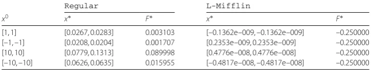
Table 3 Numerical results for “Regular” and “L-Mifflin”

Regular L-Mifflin

x0 x∗ F∗ x∗ F∗

[image:21.595.117.480.442.572.2] [image:21.595.116.479.605.674.2]

[1, 1] [0.0267, 0.0283] 0.003103 [–0.1362e–009, –0.1362e–009] –0.250000

[–1, –1] [0.0208, 0.0204] 0.001707 [0.2353e–009, 0.2353e–009] –0.250000

[10, 10] [0.0779, 0.1313] 0.089998 [0.4776e–008, 0.4776e–008] –0.250000

[–10, –10] [0.0626, 0.0635] 0.015955 [–0.4817e–008, –0.4817e–008] –0.250000

Acknowledgements

Project supported by the National Natural Science Foundation (11761013, 11771383) and Guangxi Natural Science Foundation (2013GXNSFAA019013, 2014GXNSFFA118001, 2016GXNSFDA380019) of China.

Competing interests

The authors declare that they have no competing interests.

Authors’ contributions

All authors read and approved the final manuscript. CT mainly contributed to the algorithm design and convergence analysis; JL mainly contributed to the convergence analysis and numerical results; and JJ mainly contributed to the idea of the method and algorithm design.

Author details

1_{College of Mathematics and Information Science, Guangxi University, Nanning, P.R. China.}2_{College of Science, Guangxi}

University of Nationalities, Nanning, P.R. China.

Publisher’s Note

Springer Nature remains neutral with regard to jurisdictional claims in published maps and institutional affiliations.

Received: 2 March 2018 Accepted: 28 March 2018

References

1. Chartrand, R.: Exact reconstruction of sparse signals via nonconvex minimization. IEEE Signal Process. Lett.14(10), 707–710 (2007)

2. Hare, W., Sagastizábal, C., Solodov, M.V.: A proximal bundle method for nonsmooth nonconvex functions with inexact information. Comput. Optim. Appl.63(1), 1–28 (2016)

3. Attouch, H., Bolte, J., Redont, P., Soubeyran, A.: Proximal alternating minimization and projection methods for nonconvex problems: an approach based on the Kurdyka–Łojasiewicz inequality. Math. Oper. Res.35(2), 438–457 (2010)

4. Bolte, J., Sabach, S., Teboulle, M.: Proximal alternating linearized minimization for nonconvex and nonsmooth problems. Math. Program.146, 459–494 (2014)

5. Dinh, Q.T., Diehl, M.: Proximal methods for minimizing the sum of a convex function and a composite function (2011). arXiv:1105.0276

6. Eckstein, J., Svaiter, B.F.: A family of projective splitting methods for the sum of two maximal monotone operators. Math. Program.111(1), 173–199 (2007)

7. Goldfarb, D., Ma, S., Scheinberg, K.: Fast alternating linearization methods for minimizing the sum of two convex functions. Math. Program.141, 349–382 (2013)

8. Kiwiel, K.C.: A method for minimizing the sum of a convex function and a continuously differentiable function. J. Optim. Theory Appl.48(3), 437–449 (1986)

9. Kiwiel, K.C.: An alternating linearization bundle method for convex optimization and nonlinear multicommodity flow problems. Math. Program.130(1), 59–84 (2011)

10. Li, D., Pang, L., Chen, S.: A proximal alternating linearization method for nonconvex optimization problems. Optim. Methods Softw.29(4), 771–785 (2014)

11. Mine, H., Fukushima, M.: A minimization method for the sum of a convex function and a continuously differentiable function. J. Optim. Theory Appl.33(1), 9–23 (1981)

12. Tuy, H., Tam, B.T., Dan, N.D.: Minimizing the sum of a convex function and a specially structured nonconvex function. Optimization28, 237–248 (1994)

13. Hare, W.L., Sagastizábal, C.: A redistributed proximal bundle method for nonconvex optimization. SIAM J. Optim.

20(5), 2442–2473 (2010)

14. Cheney, E.W., Goldstein, A.A.: Newton’s method for convex programming and Tchebycheff approximations. Numer. Math.1, 253–268 (1959)

15. Kelley, J.E.: The cutting-plane method for solving convex programs. J. Soc. Ind. Appl. Math.8, 703–712 (1960) 16. Hare, W., Sagastizábal, C.A.: Computing proximal points of nonconvex functions. Math. Program.116(1), 221–258

(2009)

17. Rockafellar, R.T., Wets, R.J.B.: Variational Analysis. Springer, Berlin (1998)

18. Rockafellar, R.T.: Monotone operators and the proximal point algorithm. SIAM J. Control Optim.14(5), 877–898 (1976) 19. Lemaréchal, C.: An extension of Davidon methods to nondifferentiable problems. Math. Program. Stud.3, 95–109

(1975)

20. Wolfe, P.: A method of conjugate subgradients for minimizing nondifferentiable functions. Math. Program. Stud.3, 145–173 (1975)

21. Bonnans, J.F., Gilbert, J.C., Lemaréchal, C., Sagastizábal, C.: Numerical Optimization: Theoretical and Practical Aspects, 2nd edn. Springer, Berlin (2006)

22. Kiwiel, K.C.: Methods of Descent for Nondifferentiable Optimization. Lecture Notes in Mathematics, vol. 1133. Springer, Berlin (1985)

23. Kiwiel, K.C.: A method of centers with approximate subgradient linearizations for nonsmooth convex optimization. SIAM J. Optim.18(4), 1467–1489 (2008)

24. Kiwiel, K.C.: An algorithm for linearly constrained convex nondifferentiable minimization problems. J. Math. Anal. Appl.105(2), 452–465 (1985)

26. Bagirov, A.M., Karmitsa, N., Mäkelä, M.: Introduction to Nonsmooth Optimization: Theory, Practice and Software. Springer, Cham (2014)