THE FIRST-ORDER COMPLEX ODE WITH
POLYNOMIAL NONLINEAR PART
ANDREI BORISOVICH AND WACŁAW MARZANTOWICZ
Received 8 February 2004; Revised 7 March 2004; Accepted 12 March 2004
We study nonlinear ODE problems in the complex Euclidean space, with the right-hand side being polynomial with nonconstant periodic coefficients. As the coefficients func-tions, we admit only functions with vanishing Fourier coefficients for negative indices. This leads to an existence theorem which relates the number of solutions with the num-ber of zeros of the averaged right-hand side polynomial. A priori estimates of the norms of solutions are based on the Wirtinger-Poincar´e-type inequality. The proof of existence theorem is based on the continuation method of Krasnosielski et al., Mawhin et al., and the Leray-Schauder degree. We give a few applications on the complex Riccati equation and some others.
Copyright © 2006 Hindawi Publishing Corporation. All rights reserved.
1. Introduction
This work is devoted to theC-valuedT-periodic positive orientedC1-smooth solutions of the ordinary differential equation of the form
˙
u(t)=
N
k=0
ck(t)uk(t), (1.1)
whereck(t),k=0,. . .,N, areC-valueT-periodic positive oriented continuous functions. The study of such solutions was begun in [6]. In this review article we present some new description of our results and their applications to the complex Riccati equation. Some theorems are presented in more general forms and proofs are given in more detail.
The algebra of positive orientedC-valuedT-periodic functionsC1
+(T) attracted our attention by two reasons. At first, inC1+(T) we developed a special technique of a priori estimates of solution, which does not occur in the usual algebraC1(T). These estimates give a possibility to separate and to localize the solutions and find favorable conditions for using the degree theory for their determination.
Hindawi Publishing Corporation Journal of Inequalities and Applications Volume 2006, Article ID 42908, Pages1–21
In this work we use a priori estimates of solution of two types. At first, the mean value uof solutionu(t)∈C1
+(T) is a root of the polynomial equation
0=
N
k=0
ckuk (1.2)
or, shortly 0=P(u), where the coefficients of the associated polynomialPare averaging values
ck= 1
T T
0 ck(t)dt, u= 1
T T
0 u(t)dt (1.3)
andn=degPN. Secondly, some assumptions for the coefficients of (1.1) and for their mean values lead to the following: that theC0-normu
0of solutionu(t)∈C1+(T) be-longs to the sum of two intervals [r0,r1]∪[r2, +∞), where 0r0< r1< r2. This estimate is fulfilled only in the algebra of positive oriented functions and is based on the Wirtinger and Poincare inequality (see [19] for details). We study only the first part of set of solu-tions (with norms in [r0,r1]) and prove that it is a compact subset.
InSection 2we give the definition of the Banach algebraCk
+(T) for integerk0 and the definition of the associated polynomialP(z). Next, we formulate mainTheorem 2.4. This theorem gives a sufficient condition for the existence of aT-periodic solutionu(t) withu=z0, where z0 is a root ofP(z). InSection 3 we give all properties of positive oriented functions which we need for study of (1.1).Section 4is devoted to the proof of a priori estimates.
Section 5contains the proof of main theorem on the base of the continuation method of Krasnosielski et al. and Mawhin et al. and the Leray-Schauder degree. In some sense our hypothesis is equivalent to an assumption that (1.1) is a small perturbation of (1.2) if the frequency is large enough, which resembles previous approaches to the problem [15,17,21]. However, we must say that as well our analytical framework as the required a priori bound have very natural form and lead to a multiplicity result to an effective estimate of the period.
In lastSection 6we give a few applications of our main theorem to the complex Riccati equation and make a comparison with other results in this direction (Lloyd [14], Hassan [12], Campos and Ortega [10], Miklaszewski [20], and ˙Zoła¸dek [22]). We also study the positive oriented periodic solutions on the base of the Nielsen fixed-point theory, see [1,2,7,8,11] and [3–5]. In particular, we use the theorems on multiplicity of distinct roots of a complex polynomial [4,7].
In the end, we remark that the positive oriented solutions of the equation
˙
u(t)= f(t,u) (1.4)
2. Main theorem
In this work we look for the solutionsu(t)∈C1
+(T) of nonlinear differential equation
˙
u(t)= N
k=0
ck(t)uk(t) (2.1)
withcN(t)≡0, integerN2 and coefficientsck(t)∈C+0(T) for allk=0, 1,. . .,N. Let Cp(T) for integer p0 and realT >0 denotes the Banach algebra of the Cp -smoothC-valuedT-periodic functionsu(t) with the norm
up=
p
k=0 u(k)
0, u(k)0= max t∈[0,T]
u(k)(t). (2.2)
We assign to a given functionu(t)∈C0(T) its Fourier series
u(t)∼
+∞
k=−∞
fk(u)eiνkt, ν=2π
T , (2.3)
with the coefficients
fk(u)= 1
T T
0 u(t)e
−iνktdt. (2.4)
Definition 2.1. LetC+(p T) be a set of all functionsu(t)∈Cp(T) satisfying f
k(u)=0 for all integerk <0. The subsetC+(p T) is a Banach subalgebra inCp(T). We call it the algebra of positive oriented functions.
ByA:C0(T)→Cwe denote the functional of averaging, that is, it assigns to a given functionu(t) its mean value
A(u)=T1 T
0 u(t)dt. (2.5)
Remark that the mean valueA(u) is equal to the 0th Fourier coefficient f0(u). Definition 2.2. A polynomialP(z)∈C[z] is associated with (2.1) if
P(z)=
N
k=0
ckzk, (2.6)
l(x, r0) ω(x)
l(r, r0) ω(r)
c00
−2
Tr0
r0 r1 r r2 x
(a)
l(x, r0) ω(x)
l(r, r0)=ω(r)
c00
−2
Tr0
r0 r x
(b)
Figure 2.1
Remark 2.3. If the mean valuecn=0 for a certain integer 1nNandck=0 for all integerk=n+ 1,. . .,N, then degP=n. The degree of associated polynomialP(z) is a less or equal than the degree of right part of (2.1).
We assign also to (2.1) two functionsl,ω:R+→Rdefined by formulae
lx,r0
=T2x−r0
, ω(x)=
N
k=0 ck(t)
0xk, (2.7)
depending from real variablex0. Functionl(x,r0) is depending on parameterr00 in addition. The graph ofω(x) starts from the pointω(0)= c0(t)0, it is a convex and increasing. The graph ofl(x,r0) is a direct line which starting from the pointl(0,r0)=
−(2/T)r0with the angleϕ, where tanϕ=2/T.
On Figures2.1(a) and2.1(b) the possibility intersections of the graphs ofl(x,r0) and
ω(x) are showed.
We are now in position to formulate the main theorem. Theorem2.4. Consider (2.1). Suppose that
(i)realT >0, integerN2andcN(t)=0; (ii)coefficientsck(t)∈C+(0 T)for allk=0, 1,. . .,N; (iii)mean valuecn=0for a certain integer1nN; (iv)numberz0∈Cis a root of the associated polynomialP(z);
(v)equation
ω(x)=lx,r0
2
T
ω(x)
c00
r x
Figure 2.2
wherer0= |z0|, has a two distinct roots r1< r2 in the interval[0, +∞), see Figure 2.1(a). Then (2.1) has at least one solutionu(t)∈C1
+(T)with the mean value
A(u)=z0. (2.9)
Moreover, itsC1-norm is bounded as follows
r0u(t)0r1, u˙(t)0 2
T
r1−r0. (2.10)
The proof ofTheorem 2.4will be given inSection 5. Next, we will study the equation
ω(x)=lx,r0
. (2.11)
Noter >0 a point, where the tangent line ofω(x) is a parallel tol(x,r0). The pointris not depending from the parameterr0and may be found from the equalityω(r)=tanϕ, that is
N
k=1
kck(t)0rk− 1= 2
T. (2.12)
The graph ofω(x) starts from the pointsω(0)= c1(t)0and increases. The condi-tion
c1(t) 0<
2
T (2.13)
If for a certainr00 the graphs ofω(x) andl(x,r0) have a two distinct intersection pointsr1< r2in the interval [0, +∞), thenr1< r < r2andω(r)< l(r,r0), that is
N
k=0 ck(t)
0rk< 2
T(r−r0), (2.14)
seeFigure 2.1(a). Moreover:
Property 2.5. The fulfilment of the inequalities (2.13) and (2.14) for a certainr00 is a necessary and sufficient condition for an existence in the interval [0, +∞) of the two distinct points of intersection of the graphs ofω(x) andl(x,r0).
Remark 2.6. The inequality (2.14) may be written in the form
r0< r−
T
2 N
k=0 ck(t)
0rk, (2.15)
what is a very convenient for the application to the differential equation (2.1) because the constantr0= |z0|in the left part of (2.15) depending only from the mean valuesckof the coefficients of (2.1) and the constant in the right part of the inequality (2.15) depending from itsC0-norms and periodT.
3. Algebra of periodicC+-functionsp
At first we study the properties of the Banach algebrasC+(p T), integer p0 andT >0, which are necessary for the proof of mainTheorem 2.4.
InC0(T) consider the following linear subspace of the trigonometrical polynomials
E(T)=
c0+ m
k=1
ckek(t) :c0,ck∈C,m=1, 2,. . . , (3.1)
where
e(t)=eiνt, ν=2π
T . (3.2)
It is clear, thatE(T) is a subspace of everyCp(T).
Definition 3.1. We will denote byC+(p T) the closure of subspaceE(T) inCp(T) with respect to its norm · p.
Definition 3.1is equivalent toDefinition 2.1, see [6].
We assign to a given periodT >0 the two dimensional open disc on the complex plane
Dτ=
z:|z|< τ, τ= T
Let us denote bySτits boundary and byDτthe closed disc. Remark that the length ofSτ is equal toT. For a givenC-valued functiong(z), which is defined in some open neigh-borhood ofDτ, we assign its restrictionu(t) to the boundarySτby following formula
u(t)=gτeiνt. (3.4)
Remark that the each trigonometrical polynomial
v(t)=
m
k=0
ckeiνkt (3.5)
is a restriction to the circleSτof the corresponding holomorphic function
h(z)= m
k=0
ckνk
zk. (3.6)
LetH(Dτ) denotes the linear space of theC-valued functionsh(z) defined and holo-morphic in some open neighborhood ofDτ. LetCp(Sτ) denotes the Banach algebra of theCp-smoothC-valued functionsu(t) defined on the circleS
τ. Note thatCp(Sτ) can be identified withCp(T). We callH(S
τ) orH(T) the set of restrictions to the boundarySτ of all functionsh(z)∈H(Dτ). The setH(T) is a linear subspace inCp(T) for all integer
p0.
Definition 3.2. We will denote by C+(p T) the closure of subspaceH(T) inCp(T) with respect to its norm · p.
Definition 3.2is equivalent to Definitions2.1and3.1, see [6].
Property 3.3. The functional of averagingA:C+(p T)→C, defined by (2.2), is a linear and multiplicative, that is, for everyu(t),v(t)∈C+(p T) and everyα,β∈Cwe have
A(αu+βv)=αA(u) +βA(v),
A(uv)=A(u)A(v). (3.7)
Property 3.3may be simple verified foru(t),v(t)∈E(T), see formula (3.1).Property 3.3for all functions inC+(p T) follows from the continuity ofA.
Definition 3.4. We callV+p(T), integerp0 and realT >0, the kernel subspace of the averaging functionalA:C+(p T)→Cdefined by (2.3).
Recall thatV+p(T) is a set of all functionsv(t)∈C+(p T) having f0(v)=0, where f0(v) is its 0th Fourier coefficient.
Property 3.5. The Banach algebraC+(p T), integerp0 and realT >0, may be written as a direct sum
C+(p T)=V0⊕V+p(T). (3.8)
The every functionv(t)∈V+(p T) may be written as
v(t)=eiνtu(t), (3.9)
whereu(t)∈C+(p T). Therefore, the Banach algebrasC+(p T) andV+(p T) are isometric. For a given integerm0 we have a decomposition
C+(p T)=V0⊕V1(T)⊕ ··· ⊕Vm(T)⊕V+pm(T), (3.10)
where
Vk(T)=ceiνkt:c∈C, k=0, 1,. . .,m, (3.11)
andV+pm(T) is a Banach algebra of all functionsv(t)∈C+(p T) satisfying
fk(v)=0, k=0, 1,. . .,m. (3.12)
Note that algebrasV+pm(T) in the decompositions (3.10) for all integerm0 are isomet-ric toC+(p T). Moreover,V+0p(T)=C
p
+(T) andV+1p(T)=V p +(T).
Definition 3.6. We callJ the projectorJ:C+(p T)→C+(p T) to the subspaceV0along the idealV+p(T) defined by formula
J(u)=A(u)e0. (3.13)
It is a multiplicative linear bounded map with ImJ=V0and KerJ=V+p(T) preserving all elements fromV0.
Definition 3.7. We will denote byDthe operator of derivativeD:C+(p T)→C+p−1(T), in-tegerp1 and realT >0, defined by the formula
D(u)(t)=u˙(t). (3.14)
Property 3.8. The operatorDis a linear bounded. It belongs to the classΦ0, that is, is a Fredholm map of index 0. Moreover, it has
KerD=V0, ImD=V+p−1(T). (3.15)
Property 3.9. LetA:C0
+(T)→Cdenotes the functional of averaging, see (2.2), andu(t)∈
C1
+(T). Then we have
A( ˙u)=0. (3.16)
To proveProperty 3.9consider the differential operatorD:C+(1 T)→C0+(T). We have
V+(0 T)=ImD=KerA. (3.17)
Definition 3.10. We will denote byLthe differential operatorL:C+(p T)→C+p−1(T), inte-gerp1 and realT >0, defined by the formula
L(u)(t)=u˙(t) +u(t). (3.18)
Property 3.11. The operatorLis an isomorphism.
To proveProperty 3.11we write the operatorLas a sum
L=D+E◦I, (3.19)
whereI:C+(p T)→C+(p T) is the identity map andE:C+(p T)→C+p−1(T) is a natural em-bedding of the Banach algebras. Recall thatEis a completely continuous. Following the superpositionE◦Iis a completely continuously too. In the sum (3.19) the first operator belongs to the classΦ0and the second is a completely continuous. ThereforeL∈Φ0. It is not difficult to verify that KerL= {0}. Following the mapLis an isomorphism.
4. A priori estimates of solutions inC+-algebrap
The proof of the mainTheorem 2.4is based on the homotopy
˙
u(t)=
N
k=0
λck(t)uk(t) + (1−λ)ckA(u)k
(4.1)
with parameterλ∈[0, 1], where the constantsck=A(ck) are mean values ofck(t),A(u) is a mean value ofu(t). Remark that the homotopy (4.1) is thought to deformation (2.1) to a simpler equation ˙u=P(u), wherePis a polynomial associated with (2.1). The simpler equation has only constant solutionsu(t)≡z, ˙u(t)≡0, wherez is a root ofP. In this section we will give some a priori properties of the solutions of (4.1) inC1(T) andC1
+(T), which we need to prove the mainTheorem 2.4.
We will use the following inequality of the Wirtinger-Poincare type, see [19] and [6] for details.
Property 4.1. Letu(t)∈C1(T) be aT-periodic function,u=A(u) its mean value and
u0itsC0-norm, see formulae (2.5) and (2.2). Then
0u0− |u|
T
Proof. For every 0t0Twe have
0u(t)0−u
t0u(t)−u
t00
T
2u˙(t)0. (4.3) On the other hand for the mean valueuof any periodic functionu(t)∈C1(T) we have
|u||u(t∗)|for somet∗∈[0,T]. This leads toProperty 4.1.
Property 4.2. Consider (4.1) with realT >0, integer N2 and all coefficient ck(t)∈
C0(T). Letu(t)∈C1(T) is a solution for someλ∈[0, 1]. Then the following inequality holds:
2
T
u0− |u|
N
k=0 ck
0uk0, (4.4)
or, shortly,
lu0,|u|ωu0
. (4.5)
Recall thatu=A(u) is a mean value ofu(t) and
u0= max
t∈[0,T]
u(t). (4.6)
Proof. To prove Property 4.2we calculate theC0-norms from the left and right parts of (4.1) and use the inequalities|ck|ck0 for allk=0, 1,. . .,N and |A(u)|u0. We get
u˙ 0 N
k=0 ck
0uk0 (4.7)
independently from the parameterλ∈[0, 1]. From (4.2) we get 2
T
u0− |u|
u˙ 0. (4.8)
The inequalities (4.7) and (4.8) leadProperty 4.2.
Property 4.3. Letu(t)∈C1
+(T) is a solution of (4.1) for someλ∈[0, 1], where integer
N2 and all coefficientsck(t)∈C0+(T). Then its mean valueu=A(u) is a root of the associated polynomialP(z), that is
0=
n
k=0
ckuk. (4.9)
To proveProperty 4.3we calculate the mean values from the left and right parts of (4.1) and apply Properties3.3and3.9.
Remark that (4.1) for eachλ∈[0, 1] has a same associated polynomialP(z) at degree
nN. LetP−1(0)= {z1,. . .,z
the fiberF(zj) in the spaceC1+(T) defined by formula
Fzj
=u(t) :A(u)=zj
, j=1,. . .,m. (4.10)
Note that all solutions of (4.1) in the algebraC1
+(T) belong to the setF, which is a sum of all fibers
F=Fz1
∪ ··· ∪Fzm. (4.11)
Theorem4.4. Consider the family (4.1) with parameterλ∈[0, 1]. Suppose that (i)realT >0, integerN2andcN(t)=0;
(ii)coefficientsck(t)∈C+0(T)for allk=0, 1,. . .,N;
(iii)mean valuecn=0for a certain integer1nNandck=0for allk > n; (iv)numberz0∈Cis a root of the associated polynomialP(z);
(v)functionu(t)∈C1
+(T)is a solution of (4.1) for someλ∈[0, 1]andA(u)=z0. Then, itsC0-norm and mean value satisfy a priori inequality
lu0,z0ω
u0
, (4.12)
where the functionsl(x,r0)andω(x)defined by formulae (2.7).
Theorem 4.4follows directly from Properties4.2and4.3.
Remark 4.5. If the supposition (v) of the mainTheorem 2.4is fulfilled, seeFigure 2.1(a) and Property 2.5, then for each solution u(t)∈F(z0)⊂C1
+(T) of (2.1) its C0-norm
u(t)0 belongs to the one of two intervals [r0,r1] or [r2, +∞), where r0= |z0| and
r1< r2are positive roots of the equationl(x,r0)=ω(x). If the supposition (v) of the main Theorem 2.4is not fulfilled, thenu(t)0belongs to [r0, +∞), seeFigure 2.1(b).
5. Proof of main theorem
We are now in position to prove the mainTheorem 2.4. Introduce the following operators acted in the Banach algebras of positive oriented functions:
L:C1
+(T)−→C0+(T), Lu(t)=u˙(t) +u(t), (5.1)
is an isomorphismL=D+I, seeProperty 3.11;
Q:C0
+(T)−→C0+(T), Qu(t)= N
k=0
ck(t)uk(t) +u(t), (5.2)
is a nonlinear continuous map (evaluation Niemytskij operator);
E:C1
is a natural embedding of the Banach algebras (completely continuous map);
J:C1
+(T)−→C+1(T), Ju(t)=A(u)e0(t), (5.4) is a projector to the subspaceV0∼C, wheree0(t)≡1 is an element ofC1+(T).
Reduce the differential equation (2.1) to a fixed point problemu=G(u) with the com-pletely continuous mapG:C+(1 T)→C1+(T). Add the functionu(t) to the left and right parts of (2.1). We get
˙
u(t) +u(t)=
N
k=0
ck(t)uk(t) +u(t). (5.5)
Equation (5.5) may be written in the operator form
L(u)=Q◦E(u), (5.6)
where the operatorsL,Q,Eare defined by (5.1), (5.2), and (5.3). Equation (5.6) may be written in the form
u=L−1◦Q◦E(u) (5.7)
with the help of the invertibility ofL, seeProperty 3.11. Denote
G=L−1◦P◦E. (5.8)
Then, the operator equation (5.7) or differential equation (2.1) may be written as a fixed points problemu=G(u) for the completely continuous mapG:C1
+(T)→C1+(T) defined by formula (5.8). The mapG is a completely continuous because one of the elements of decomposition (5.8) is a completely continuous embedding of the Banach algebras, see (5.3).
The actions of all operators are illustrated on the following scheme
C1+(T) L
−→C0+(T) Q
←−C+0(T) E
←−C+1(T). (5.9)
Recall that the proof of the mainTheorem 2.4is based on the homotopy (4.1), which is thought to deform (2.1) to a simpler equation. Write all of this equations together:
˙
u(t)=
N
k=0
ck(t)uk(t), λ=1,
˙
u(t)= N
k=0
λck(t)uk(t) + (1−λ)ckA(u)k
, 0λ1,
˙
u(t)=
N
k=0
ckA(u)k, λ=0.
Write this homotopy in the operator form:
u=G(u), λ=1,
u=Gλ(u), 0λ1,
u=J◦G(u), λ=0.
(5.11)
Recall, seeProperty 3.5, that the Banach algebraC+(1 T) may be written as a direct sum
C+(1 T)=V+(1 T)⊕V
0 (5.12)
with the finite-dimensional subspace
V0=
Ce0(t) :C∈C∼C, (5.13)
wheree0(t)≡1 is an element ofC1+(T). The mapJ:C1+(T)→C1+(T) is a projector toV 0 alongV1
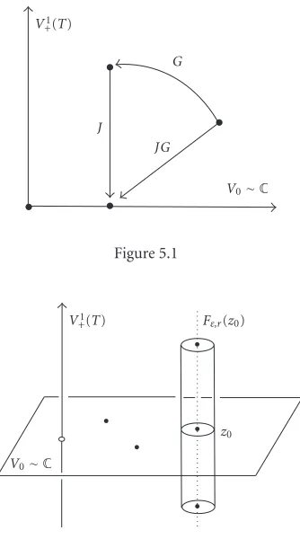
+(T), seeDefinition 3.6. Following the operatorJ◦G:C1
+(T)→C+1(T) acts by right
J◦G(u)(t)= N
k=0
ckA(u)k+A(u)
e0(t) (5.14)
and it has a finite-dimensional image, seeFigure 5.1. All its fixed points belong to the finite-dimensional subspace, that is
Im(J◦G)⊂V0, Fix(J◦G)⊂V0. (5.15)
FromDefinition 2.2of the associated polynomialP(z),Property 4.3and the equality (5.14) we get
(J◦G−I)V0∼C=P, (5.16)
where the left part of (5.16) is a restriction of the mapJ◦G−Ito the finite-dimensional subspaceV0. On the base of (5.16) we get
Fix (J◦G)=P−1(0) (5.17)
or, more exactly, the equation
u=J◦G(u) (5.18)
is equivalent to the system
u(t)≡z, z∈C,
P(z)=0, P:C−→C. (5.19)
Property 5.1. Consider the family of (5.11) with parameterλ∈[0, 1]. Let the number
V1 +(T)
J
G
JG
[image:14.468.151.318.72.382.2]V0∼C
Figure 5.1
V1
+(T) Fε,r(z0)
z0
V0∼C
Figure 5.2
Recall, seeProperty 4.3andFigure 5.2, that this solution belongs to the fiber
Fz0
=u(t) :A(u)=z0
. (5.20)
We would like to show on the base of the Leray-Schauder degree that the root ofu=Gλ(u) will be preserved in the fiberF(z0) for allλ∈[0, 1].
Now, we are in position to apply the Leray-Schauder degree. Lemma5.2. LetUis a bounded open connected set inC1
+(T). Consider the intersection
UC=U∩V0. (5.21)
Assume thatUC= ∅, then it is a bounded open connected set inV0∼C. Suppose that the boundary∂UCthere is not a roots of the associated polynomialP(z). Then,
deg (J◦G−I,U, 0)=degP,UC, 0, (5.22)
Choose the sufficiently small open neighborhood ofz0inC
Cεz0
=z:z−z0< ε
, (5.23)
such that its closure does not consist others roots of the associated polynomialP(z). Choose also the real number r >0 such that r1 < r < r2, see supposition (v) of Theorem 2.4andFigure 2.1(a). For example,rmay be chosen as a unique root of (2.12).
In Banach algebraC+(1 T) define the open bounded connected set by following
Fε,r
z0
=
u(t) :A(u)−z0< ε,u0< r,u˙ 0< N
k=0 ck
0rk , (5.24)
seeFigure 5.2. Remark that
Fε,r
z0
∩V0=Cε
z0
. (5.25)
For each solutionu(t)∈F(z0)⊂C1
+(T) of the equationu=Gλ(u) for someλ∈[0, 1] its
C0-normu(t)
0belongs to the one of two intervals [r0,r1] or [r2, +∞). It follows from Theorem 4.4and supposition (v) ofTheorem 2.4. We get
u0r1< r or r < r2u0. (5.26)
From (5.26) andProperty 4.3we get
FixGλ∩∂Fε,rz0= ∅ (5.27)
for allλ∈[0, 1].
Finally. Letz0∈Cis a root of the associated polynomialP(z). Then:
degP,Cεz0
, 0=0;
u0(t)≡z0is a solution ofu=J◦G(u);
u0(t) belongs to the setFε,r
z0
.
(5.28)
Using the Leray-Schauder degree andLemma 5.2, we get
degI−G,Fε,r
z0
, 0=degI−Gλ,Fε,r
z0
, 0
=degI−J◦G,Fε,r
z0
, 0
=deg−P,Cεz0
, 0=0.
(5.29)
Following the equationu=G(u) has at least one solutionu(t)∈Fε,r(z0)⊂C1+(T).
6. Applications
Property 6.1. On the complex plane consider the following polynomial equation
0= n
k=0
ckzk, (6.1)
where all coefficientck∈C, integer 0kn, andcn=0. Denote
m=|1
cn| n−1
k=0
ck. (6.2)
Then, each rootz0of (6.1) is satisfied to one of two following a priory estimates
z0m1/n, ifm<1, (6.3)
or
z0m, ifm1. (6.4)
FromTheorem 2.4,Property 2.5,Remark 2.6, andProperty 6.1we get following the-orem.
Theorem6.2. Consider the differential equation (2.1). Suppose that (i)realT >0, integerN2andcN(t)≡0;
(ii)coefficientsck(t)∈C+(0 T)for allk=0, 1,. . .,N; (iii)C0-normc1(t)
0<2/T;
(iv)mean valuecn=0for a certain integer1nNandck=0forn < kN; (v)one of the two following inequalities holds
m1/n< r−T 2
N
k=0 ck(t)
0rk, ifm<1, (6.5)
or
m< r−T
2 N
k=0 ck(t)
0rk, ifm1, (6.6)
wherer >0is a unique root of (2.12) andm0is defined by (6.2). Then, for each root
z0 of the associated polynomialP(z)correspond at least one solution u(t)∈C1+(T)of the differential equation (2.1) with the mean valueA(u)=z0andC0-norm less thanr.
The proof ofTheorem 6.2is based on the fact, that the inequality (6.5) or (6.6) leads the inequality (2.14) or (2.15) for all roots of associated polynomialP(z) simultaneously. Remark 6.3. The supposition (iv) implies that degP=n.
We will give a sufficient condition for the existence inC1
Theorem6.4. Consider the differential equation (2.1). Let supposition(i)–(v) ofTheorem 6.2are fulfilled. Assume that all coefficientsck, 0kn, satisfy the conditions
c0>c1+c2+···+cs,
cs+1>c0+···+cs+cs+2+···+cn, (6.7)
for a certain integer 1sn. Then, the differential equation (2.1) has at leastsdistinct solutions in the algebraC1
+(T) withC0-norm less thanr.
The statement follows fromTheorem 6.2and example to corollary and proposition 3 of [8]. The fulfilment of (6.7) is a sufficient condition for the existence ofsdistinct roots of the associated polynomialP(z). This fact was proved in [8] on the base of the Nielsen Fixed Point Theory, see also [7] and [11].
Property 6.5. On the complex plane consider the polynomial equation
0=zn+ n−1
k=0
ckzk, (6.8)
where all coefficientck∈C, integer 0kn−1. If
1 +c0+n−1 k=1
ck<1
2, (6.9)
Then, (6.8) hasndistinct rootsz1,. . .,znsuch that
1 2
1/n
zj1 +1
2, j=1,. . .,n. (6.10)
Property 6.5follows from Theorem 2.1 in [4], which was proved on the base of Nielsen Fixed Point Theory (see also [3,5]).
FromTheorem 6.2andProperty 6.5we get the following theorem. Theorem6.6. Consider the differential equation (2.1). Suppose that
(i)realT >0, integerN2andcN(t)≡0; (ii)coefficientsck(t)∈C+0(T)for allk=0, 1,. . .,N; (iii)C0-normc1(t)
0<2/Tandr >0is a unique root of (2.12); (iv)following inequality holds
3 2< r−
T
2 N
k=0 ck(t)
0rk; (6.11)
(v)mean valuecn=1for a certain integer1nNandck=0forn < kN; (vi)following inequality holds
1 +c0+n−1 k=1
ck<1
Then, (2.1) has at leastndistinct solutions in the Banach algebraC1
+(T)withC0-norm less thanr.
Theorem 6.6is a very convenient for applications because the verification of assump-tions (iii) and (iv), which connected withC0-norm of coefficients and periodT, is sep-arated from the verification of assumptions (v) and (vi), which connected with its mean values.Theorem 6.6may be applied to the differential equations in the form
˙
u(t)=un(t) + n−1
k=0
ck(t)uk(t), (6.13)
wherecn(t)≡cn=1 andn=N=degP. Such equations were studied by many authors (see, for example, [9,10,13,14,17,18,20] and some others).
Example 6.7. Let us consider the complex equation ˙
u=un+c(t), (6.14)
wherec(t)∈C0
+(T) for given periodT >0 and integern2. Remark then forn=2 it is the Riccati equation.
Apply the mainTheorem 2.4. We need to verify the assumption (v). Let nextc∈Cis a mean value ofc(t). Then, the associated polynomialP(z)=zn+c. Ifc=0, then it hasn distinct complex rootsz1,. . .,znand
r0=zi= |c|1/n. (6.15)
Ifc=0, then the associated polynomialP(z)=znhas only one rootz
0=0. The functions
ω(x) andl(x,r0) defined by formulae
ω(x)=xn+c0, lx,r0= 2
T
x−r0. (6.16)
For the verification of the assumption (v) we will useProperty 2.5. Find out the rootr >0 of the equationω(r)=2/T. We get
r= 2 nT
1/(n−1)
. (6.17)
The inequalityc10<2/Tis fulfilled becausec10=0. The inequalityω(r)< l(r,r0) in the case of (6.14) has a following form:
rn+c 0< 2
T
r−r0
. (6.18)
After some calculations, we get a following theorem. Property 6.8. Consider (6.14) with the coefficientc(t)∈C0
+(T) for given periodT >0 and integern2. Ifc=0 and the following inequality holds
c0+ 2
T|c|
1/n<(n−1) 2
nT n/(n−1)
then (6.14) has at leastndistinct solutions in the algebraC1
+(T) with mean valuesz1,. . .,zn andC0-norm less thanr. Ifc=0 and
c0<(n−1)
2
nT n/(n−1)
, (6.20)
then (6.14) has at least one solution in the algebraC1
+(T) with mean value 0 andC0-norm less thanr.
Example 6.9. Let us consider (6.14) forn=2 (Riccati equation) ˙
u(t)=u2(t) +c(t), (6.21)
where the coefficient
c(t)=Reiνt±r2 0, ν=
2π
T , (6.22)
belongs to the algebraC0
+(T) for given periodT >0. Assume that realR,r0>0. Then,
c(t)0=RandP(z)=z2±r02.
Remark 6.10. Ifn=2, thenr=1/Tand the inequality (6.19) has a very simple form
R+ 2
Tr0<
1
T2. (6.23)
The inequality (6.23) is a sufficient condition for existence of two distinct solutions in the Banach algebraC1
+(T) of (6.21) withC0-norm less thanr=1/T.
Remark that all examples of (6.14) with periodicc(t) but without any periodic so-lution as these given by Lloyd [13], Hassan [12], and Campos and Ortega [10] have to be constructed withc(t) being a function outside the algebraC0
+. Indeed in all the men-tioned examplesc(t) is a real periodic function, that is,c:R→R⊂C. On the other hand we have a direct observation.
Remark 6.11. Suppose that a functionu(t)∈C+(0 T) is a real-valued. Thenu(t) is a con-stant function.
Example 6.12. In [20], by use of the Fourier series, Miklaszewski showed (under a con-jecture) that there existsR=R0>0 such that the Riccati equation
˙
u(t)=u2(t) +Reit (6.24)
has not 2π-periodic solution. Here c(t)=Reit belongs toC0+(2π) butc=0. Write the inequality (6.23) forT=2πandr0=0. We get
R < 1
4π2 (6.25)
a sufficient condition for an existence of the solutionu(t)∈C1
+(2π) of (6.24) with
A(u)=0, u0
1 2π−
1
Acknowledgment
The Research was supported by Poland Grant KBN no. 2 PO3A 045 22.
References
[1] J. Andres,A nontrivial example of application of the Nielsen fixed-point theory to differential
sys-tems: problem of Jean Leray, Proceedings of the American Mathematical Society128(2000), no. 10, 2921–2931.
[2] J. Andres, L. G ´orniewicz, and J. Jezierski,A generalized Nielsen number and multiplicity results for differential inclusions, Topology and its Applications100(2000), no. 2-3, 193–209.
[3] A. Borisovich, Z. Kucharski, and W. Marzantowicz,Nielsen numbers and lower estimates for the number of solutions to a certain system of nonlinear integral equations, Applied Aspects of Global Analysis, Novoe Global. Anal., vol. 14, Voronezh University Press, Voronezh, 1994, pp. 3–10, 99.
[4] ,Some applications of the Nielsen number to algebraic sets, Proceedings of the Conference “Topological Methods in Nonlinear Analysis”, December 1995, Gda ´nsk Scientific Society Press, Gda ´nsk, 1997, pp. 78–90.
[5] ,A multiplicity result for a system of real integral equations by use of the Nielsen number, Nielsen Theory and Reidemeister Torsion (Warsaw, 1996), Banach Center Publ., vol. 49, Polish Academy of Sciences, Warsaw, 1999, pp. 9–18.
[6] A. Borisovich and W. Marzantowicz,Multiplicity of periodic solutions for the planar polynomial equation, Nonlinear Analysis. Theory, Methods & Applications. An International Multidisci-plinary Journal. Series A: Theory and Methods43(2001), no. 2, 217–231.
[7] R. F. Brown,Retraction methods in Nielsen fixed point theory, Pacific Journal of Mathematics115 (1984), no. 2, 277–297.
[8] ,Topological identification of multiple solutions to parametrized nonlinear equations, Pa-cific Journal of Mathematics131(1988), no. 1, 51–69.
[9] J. Campos,M¨obius transformations and periodic solutions of complex Riccati equations, The Bul-letin of the London Mathematical Society29(1997), no. 2, 205–215.
[10] J. Campos and R. Ortega,Nonexistence of periodic solutions of a complex Riccati equation, Dif-ferential and Integral Equations. An International Journal for Theory & Applications9(1996), no. 2, 247–249.
[11] M. Feˇckan,Nielsen fixed point theory and nonlinear equations, Journal of Differential Equations 106(1993), no. 2, 312–331.
[12] H. S. Hassan,On the set of periodic solutions of differential equations of Riccati type, Proceedings of the Edinburgh Mathematical Society. Series II27(1984), no. 2, 195–208.
[13] N. G. Lloyd,The number of periodic solutions of the equationz˙=zN+p
1(t)zN−1+···+pN(t), Proceedings of the London Mathematical Society. Third Series27(1973), 667–700.
[14] ,On a class of differential equations of Riccati type, Journal of the London Mathematical Society. Second Series10(1975), 1–10.
[15] R. Man´asevich, J. Mawhin, and F. Zanolin,H¨older inequality and periodic solutions of some planar polynomial differential equations with periodic coefficients, Inequalities and Applications, World Sci. Ser. Appl. Anal., vol. 3, World Scientific, New Jersey, 1994, pp. 459–466.
[16] W. Marzantowicz,Periodic solutions of nonlinear problems with positive oriented periodic
coeffi-cients, Variational and Topological Methods in the Study of Nonlinear Phenomena (Pisa, 2000), Progr. Nonlinear Differential Equations Appl., vol. 49, Birkh¨auser Boston, Massachusetts, 2002, pp. 43–63.
[18] ,Continuation theorems and periodic solutions of ordinary differential equations, Topo-logical Methods in Differential Equations and Inclusions (Montreal, PQ, 1994), NATO Adv. Sci. Inst. Ser. C Math. Phys. Sci., vol. 472, Kluwer Academic, Dordrecht, 1995, pp. 291–375. [19] J. Mawhin and M. Willem,Critical Point Theory and Hamiltonian Systems, Applied Mathematical
Sciences, vol. 74, Springer, New York, 1989.
[20] D. Miklaszewski,An equationz˙=z2+p(t)with no2π-periodic solutions, Bulletin of the Belgian Mathematical Society. Simon Stevin3(1996), no. 2, 239–242.
[21] R. Srzednicki,On periodic solutions of planar polynomial differential equations with periodic
coef-ficients, Journal of Differential Equations114(1994), no. 1, 77–100.
[22] H. ˙Zoła¸dek,The method of holomorphic foliations in planar periodic systems: the case of Riccati equations, Journal of Differential Equations165(2000), no. 1, 143–173.
Andrei Borisovich: Institute of Mathematics, University of Gda ´nsk, ul. Wita Stwosza 57, 80-952 Gda ´nsk, Poland
E-mail address:[email protected]
Wacław Marzantowicz: Faculty of Mathematics and Computer Science,
Adam Mickiewicz University of Pozna ´n, ul. Umultowska 87, 61-614 Pozna ´n, Poland