An accelerating algorithm for globally solving nonconvex quadratic programming

(1)

R E S E A R C H

Open Access

An accelerating algorithm for globally

solving nonconvex quadratic programming

Li Ge

1,2*

_{and Sanyang Liu}

1

*_{Correspondence:}

[email protected]

1_{School of Mathematics and}

Statistics, Xidian University, Xi’an, China

2_{School of Mathematical Sciences,}

Henan Institute of Science and Technology, Xinxiang, China

Abstract

To globally solve a nonconvex quadratic programming problem, this paper presents an accelerating linearizing algorithm based on the framework of the

branch-and-bound method. By utilizing a new linear relaxation approach, the initial quadratic programming problem is reduced to a sequence of linear relaxation programming problems, which is used to obtain a lower bound of the optimal value of this problem. Then, by using the deleting operation of the investigated regions, we can improve the convergent speed of the proposed algorithm. The proposed algorithm is proved to be convergent, and some experiments are reported to show higher feasibility and eﬃciency of the proposed algorithm.

Keywords: Nonconvex quadratic programming; Global optimization; Linear relaxation approach; Deleting technique; Branch and bound

1 Introduction

In this paper, we consider the following nonconvex quadratic programming problem (NQP):

(NQP) :

⎧ ⎨ ⎩

minf(y) =cTy+yTQy

s.t. y∈Y0₌_{_y_∈_Rn_|_Ay_≤_b_}_,

whereQ= (qjk)n×nis a realn×nsymmetric matrix;A= (ajk)m×nis a realm×nmatrix, andc,y∈Rn_;_b_∈_Rm_.

The (NQP) is an important class of global optimization problems, and it is not only because they have broad applications in the ﬁelds of statistics and design engineering, optimal control, economic equilibria, ﬁnancial management, production planning, com-binatorial optimization, and so on [1,2], but also because many other nonlinear problems can be transformed into this form [3–7], such as the following linear multiplicative pro-gramming (LMP) problem:

(LMP) :

⎧ ⎨ ⎩

minf(y) =p_i₌₁(c_iTy+di)(eT_iy+fi)

s.t. y∈Y0₌_{_y_∈_Rn_|_Ay_≤_b_}_,

(2)

wherep≥0,cT

i = (c1,c2, . . . ,cn),eTi = (e1,e2, . . . ,en)∈Rn;A= (ajk)m×nis a realm×nmatrix, anddi,fi∈R,i= 1, 2, . . . ,n;b∈Rm. Obviously, the (LMP) can be easily transformed into the (NQP). So, the applications of the (NQP) also include all the applications of the (LMP). In the last decades, many solution methods have been developed for globally solv-ing the (NQP) and its special forms. For example, branch-and-cut algorithm [8] and branch-and-bound algorithm [9] for box-constrained nonconvex quadratic programs; two efficient algorithms for linear constrained quadratic programming (LCQP) by Cam-bini et al. [10] and Li et al. [11]; branch-and-reduce approach by Gao et al. [12]; fi-nite branch-and-bound approach by Burer and Vandenbussche [13]; branch-and-bound method based on outer approximation and linear relaxation by Al-Khayyal et al. [14]; two simplicial branch-and-bound algorithms by Linderoth [15] and Raber [16]; branch-and-cut algorithm by Sherali et al. [17] and Audet et al. [18], and so on. In addi-tion, a branch-and-bound algorithm for finding a global optimal solution for a non-convex quadratic program with non-convex quadratic constraints has been proposed by Cheng Lu et al. [19]; based on the different properties of a quadratic function, five different branch-and-bound approaches for solving the (NQP) have been proposed in Refs. [20–24].

Based on the above-mentioned methods, we will present an accelerating algorithm for eﬀectively solving the (NQP) in this paper. Firstly, we present a new linear relaxation tech-nique, which can be used to construct the linear relaxation programming (LRP) of the (NQP). In addition, we divide the initial feasible region into a number of sub-regions and use deleting techniques to reduce the scope of the investigation. Then, the initial problem (NQP) is converted into a series of linear relaxation programming subproblems. We can prove that the solutions of these subproblems can converge to the global optimal value of the original problem (NQP). Finally, numerical results and comparison with the methods mentioned in recent literature show that our algorithm works as well as or better than those methods.

This paper is organized as follows. In Sect.2, we describe a new linear relaxation ap-proach for establishing the linear relaxation programming of the (NQP). In Sect.3, a range deleting technique is given for improving the convergent speed of the proposed algorithm, then a range division and deleting algorithm is proposed and its convergence is proved. Some numerical experiments are reported to show the feasibility and eﬀectiveness of our algorithm in Sect.4.

2 New linear relaxation approach

In this section, we will show how to construct the (LRP) for the (NQP). Let theith row of the matrixQbeQi, and letzi=Qiy=

n

k=1qikyk,i= 1, 2, . . . ,n, we obtain

z= (z1,z2, . . . ,zn)T= (Q1y,Q2y, . . . ,Qny)T=Qy.

By introducing new variableszi,i= 1, 2, . . . ,n, the functionf(y) can be expressed as fol-lows:

f(y,z) =cTy+yTz= n

i=1

ciyi+ n

i=1

(3)

and the setDis deﬁned as

D=y|Ay≤b,y∈Rn.

We compute the initial variable bounds by solving the following linear programming prob-lems:

y0

i =miny∈Dy, y

0

i =max

y∈D y, i= 1, 2, . . . ,n,

z0_i =min

y∈DQiy, z

0

i =max

y∈D Qiy, i= 1, 2, . . . ,n,

and let

Y0=y∈Rn|y0

i ≤yi≤y

0

i,i= 1, 2, . . . ,n

,

Z0=z∈Rn|z0_i ≤zi≤z0_i,i= 1, 2, . . . ,n,

0=(y,z)∈R2n|y0

i ≤yi≤y

0

i,z0i ≤zi≤z0i,i= 1, 2, . . . ,n

.

Based on the above discussion, we can transform the initial problem into the following equivalent problem (EP):

(EP) :

⎧ ⎪ ⎪ ⎪ ⎪ ⎪ ⎨ ⎪ ⎪ ⎪ ⎪ ⎪ ⎩

minf(y,z) =_in₌₁ciyi+n_i₌₁yizi

s.t. Ay≤b,

zi=n_k₌₁qikyk,i= 1, 2, . . . ,n,

(y,z)∈0.

For globally solving the (NQP), the computation of lower bounds for this problem and its subdivided subproblems is the principal operation in the establishment of a branch-and-bound procedure. A lower branch-and-bound on the optimal value of the (NQP) and its subdivided subproblems can be gotten by solving a linear relaxation programming of the (EP), which can be derived by a new linear relaxation approach.

Let

Y=y∈Rn_|_–_{∞ ≤}_y

i≤yi≤yi≤+∞,i= 1, 2, . . . ,n

⊆Y0, Z=z∈Rn|–∞ ≤z_i≤zi≤zi≤+∞,i= 1, 2, . . . ,n

⊆Z0

for anyy∈Y,z∈Z,i∈ {1, 2, . . . ,n}, deﬁne the functions

ϕ(yi) =y2_i, ϕl(yi) = (y

i+yi)yi– (y

i+yi)

2

4 ,

ϕu(yi) = (y

i+yi)yi–yiyi,

ϕ(zi) =z2_i, ϕl(zi) = (z_i+zi)zi–(zi+zi)

2

4 ,

(4)

ϕl(yi,zi) = 1 2

(y

i+yi)zi+ (zi+zi)yi– (y

i+yi+zi+zi)

2

4 +yiyi+zizi

,

ϕu(yi,zi) =1 2

(y

i+yi)zi+ (zi+zi)yi– (yi+zi)(yi+zi) + (y

i+yi)

2

4 +

(z_i+zi)2 4

.

Since ϕ(yi) =y2

i is a convex function ofyi over [yi,yi], its aﬃne concave envelope is

ϕu(yi) = (yi+yi)yi–yiyi. Moreover, the tangential supporting function forϕ(yi) is parallel

with theϕu(yi), thus the point of tangential support will occur atyi+₂yi, and the

correspond-ing tangential supportcorrespond-ing function isϕl(yi) = (yi+yi)yi–(yi+yi) 2

4 . Hence, by the geometric

property of the functionϕ(yi), we have

ϕl(yi) = (yi+yi)yi–

(yi+yi)2

4 ≤y

2

i ≤(yi+yi)yi–yiyi=ϕu(yi). (1) Similarly, it follows that

ϕl(zi)≤ϕ(zi)≤ϕu(zi).

Furthermore, assume that (yi+zi) is a single variable, then (yi+zi)2is a convex function about the univariate variable (yi+zi) over the interval [yi+zi,yi+zi]. By the conclusion above, we have

(yi+zi+yi+zi)(yi+zi) –(yi+zi+yi+zi)

2

4 ≤(yi+zi)

2 ₍₂₎

and

(yi+zi)2≤(yi+zi+yi+zi)(yi+zi) – (yi+zi)(yi+zi). (3)

By (1)–(3), we can obtain

ϕ(yi,zi) = 1 2

(yi+zi)2–y2i –z

2

i

≥1

2

(y

i+zi+yi+zi)(yi+zi) – (y

i+zi+yi+zi)

2

4

–1 2

(y

i+yi)yi–yiyi+ (zi+zi)zi–zizi

= 1 2

(y

i+zi+yi+zi)

2

4 +yiyi+zizi

=ϕl(yi,zi),

and

ϕ(yi,zi) = 1 2

(yi+zi)2–y2i –y2k

≤1

2

(y

i+zi+yi+zi)(yi+zi) – (yi+zi)(yi+zi)

(5)

–1 2

((y

i+yi)yi– (y

i+yi)

2

4 + (zi+zi)zi–

(z_i+zi)2

4

= 1 2

(y

i+yi)zi+ (zi+zi)yi– (yi+zi)(yi+zi) + (y

i+yi)

2

4 +

(z_i+zi)2 4

=ϕu(yi,zi).

Hence, we have

ϕl(yi,zi)≤ϕ(yi,zi)≤ϕu(yi,zi). (4)

Furthermore, we deﬁne the diﬀerence functions as follows:

(yi) =ϕ(yi) –ϕl(yi), ∇(yi) =ϕu(yi) –ϕ(yi),

(zi) =ϕ(zi) –ϕl(zi), ∇(zi) =ϕu(zi) –ϕ(zi),

(yi,zi) =ϕ(yi,zi) –ϕl(yi,zi), ∇(yi,zi) =ϕu(yi,zi) –ϕ(yi,zi).

Since(yi) is convex aboutyi, for anyyi∈[yi,yi], it follows that(yi) can attain the max-imum at the pointyioryi. Then

max

yi∈[yi,yi](yi) =ϕ(yi) –ϕ

l₍_yi_{) =}_ϕ₍_yi_{) –}_ϕl₍_yi_{) =}(yi–yi)

2

4 .

On the other hand, since∇(yi) is concave aboutyi, for anyyi∈[yi,yi],∇(yi) can attain the maximum at the point yi+₂yi, i.e.,

max

yi∈[yi,yi]∇(yi) =ϕ

u

_y

i+yi 2

–ϕ

_y

i+yi 2

=(yi–yi)

2

4 .

So, we have

max

yi∈[y_i,yi]

(yi) = max

yi∈[y_i,yi]

∇(yi)→0, as|y_i–y

i| →0, (5) that is,(yi),∇(yi)→0, asy–y →0.

Similarly, we can prove that

max

zi∈[zi,zi]

(zi) = max

zi∈[zi,zi]

∇(zi)→0, as|zi–z_i| →0, (6)

and(zi),∇(zi)→0, asz–z →0. Deﬁne

(yi+zi) = (yi+zi)2–

(y

i+yi+zi+zi)(yi+zi) – (y

i+yi+zi+zi)

2

4

,

(6)

Using the similar method, we can get the following conclusions:

max (yi+zi)∈[(y

i+zi),(yi+zi)]

(yi+zi)

= max

(yi+zi)∈[(y_i+zi),(yi+zi)]

∇(yi+zi)→0, asy–y →0,z–z →0. (7)

Since

(yi,zi) =ϕ(yi,zi) –ϕl(yi,zi)

=yizi–1 2

(y

i+yi+zi+zi)

2

4 +yiyi+zizi

= 1 2

(yi+zi)2–y2_i –y2_k

–1 2

(y

i+yi+zi+zi)

2

4 +yiyi+zizi

= 1 2

(yi+zi)2–

(y

i+yi+zi+zi)(yi+zi) – (y

i+yi+zi+zi)

2

4

+1 2

(y

i+yi)yi–yiyi–y

2

i

+(z_i+zi)zi–z_izi–z2_i

= 1

2(yi+zi) + 1 2∇(yi) +

1 2∇(zi)

≤ 1

2(yi+zi)∈[(maxy_i+zi),(yi+zi)]

(yi+zi) +1 2yimax∈[y_i,yi]

∇(yi) +1 2zimax∈[zi,zi]

∇(zi),

by (5)–(7), we can get that

(yi,zi)→0, asy–y →0,z–z →0. (8)

Similarly, we can prove that∇(yi,zi)→0, asy–y →0,z–z →0.

For convenience, without loss of generality, for anyy∈Y⊆Y0_,_z_∈_Z_⊆_Z0_{, deﬁne}

fL(y,z) = n

i=1

ciyi+ n

i=1

ϕl(yi,zi).

By utilizing the convexity of a univariate quadratic function, we establish an eﬀective method for generating the linear underestimation and linear overestimation of the func-tionsy2_i,z2_i, andyizi, respectively. By the conclusions above, the linear relaxation underesti-mation functionfL₍_y_,_z_{) of the function}_f₍_y_,_z_{) for the (EP) can be established. Thus, by the} former discussions, we can construct the corresponding approximation linear relaxation programming (LRP) of the (EP) as follows:

(LRP) :

⎧ ⎪ ⎪ ⎪ ⎪ ⎪ ⎨ ⎪ ⎪ ⎪ ⎪ ⎪ ⎩

minfL₍_y_,_z_{) =}n i=1ciyi+

n

i=1ϕl(yi,zi)

s.t. Ay≤b,

zi=n_k₌₁qikyk,i= 1, 2, . . . ,n,

(7)

By (4), it is obvious that

yizi–ϕl(yi,zi)≥0,

then

f(y,z) –fL(y,z)

= n

k=1

ciyi+ n

k=1

yizi–

_n

k=1

ciyi+ n

k=1

ϕl(yi,zi)

= n

k=1

yizi–ϕl(yi,zi)

≥0.

Thus, we havef(y,z) –fL₍_y_,_z₎_≥_{0, i.e.,}_f₍_y_,_z₎_≥_fL₍_y_,_z_). Furthermore, we have

f(y,z) –fL(y,z) = n

k=1

yizi–ϕl(yi,zi)

= n

k=1

(yi,zi).

By (8), we have that(yi,zi)→0, asy–y →0,z–z →0. Therefore, we have that

f(y,z) –fL(y,z)→0 asy–y →0,z–z →0.

Remark1 From above, we only need to solve the (LRP) instead of solving the (EP) to obtain the lower and upper bounds of the optimal value in problem (NQP).

Remark2 Based on the construction of the (LRP), each feasible point of the (NQP) in the sub-rangeis also feasible to LRP, and the global minimum value of LRP is not more than that of the (NQP) in the sub-range. Thus, the (LRP) can provide a valid lower bound for the global optimum value of problem NQP in the sub-range.

Remark3 The conclusions above ensure that the linear relaxation programming LRP can inﬁnitely approximate the (NQP), asY →0 (obviously,Z →0), this will guarantee the global convergence of the proposed algorithm.

3 Accelerating branch-and-bound algorithm and its convergence

(8)

3.1 Branching process

The critical operation of the branching process is iteratively subdividing the initial range

0into some sub-ranges, each sub-range denoted byis concerned with a node of the branch and bound, such that any inﬁnite iterative sequence of partition sets shrinks to a singleton. Here, we will adopt a standard range bisection approach, which is adequate to ensuring global convergence of the proposed algorithm. Detailed process is described as follows.

For any selected sub-range ∈ 0, Y= [y,y]⊆ Y0_{, let} _q_∈ _{arg max}_{_y

i –y_i : i= 1, 2, . . . ,n}, andym= (y

q+y

q)/2, then divideinto two sub-ranges1and2 by

sub-dividing the interval [y q,y

q] into two subintervals [y_q,ym] and [ym,yq].

From the above branching operation, we can notice that the intervals [z,z] ofz will never be partitioned by the branching processes. Hence, these branching operations only occur in a space of dimensionn, i.e., the proposed algorithm economizes the required computations.

3.2 Range deleting technique

At thekth iteration of the algorithm, for any rectanglek⊆0, we want to check whether

kcontains a global optimal solution of the (EP)(0), where

k=k₁×k₂× · · · ×k_q_–1×k_q×k_q₊₁× · · · ×k_n, with

k_q=(yq,zq)∈R2|yk q≤y

k

q≤ykq,zq0≤z0q≤z0q

.

Theorem 3.1 Assume that f is a known upper bound of the optimal value v of the(EP),for any sub-rangek_⊆0_,_{the following conclusions hold}_{: (}_i₎_{If ELB}k_>_f_,_{then there is no global} optimal solution for the(EP)overk_{; (}_ii₎_{If ELB}k_≤_f_,_{then we have}_:_{for any}_τ_{∈ {}_{1, 2, . . . ,}_n_}_, if cτ > 0,then the sub-range

k

does not contain any global optimal solution of the(EP);

else if cτ< 0,then the sub-range

k

does not contain any global optimal solution of the(EP), where

ELBk= n

i=1

minciyk i,ciy

k i

+ n

i=1 minyk

iz

0

i,yk_iz0i,yikz0i,ykiz0i

,

ρ_τk=f–RLB

k₊_min_{_c

τyk_τ,cτykτ}

cτ

, τ= 1, . . . ,n,

k=k₁×k₂× · · · ×k_τ_–1×k_τ×k_τ₊₁× · · · ×k_n,

k=k₁×k₂× · · · ×kτ–1×

k

τ×kτ+1× · · · ×kn, with

k_τ=(yτ,zτ)∈R2|ρkτ≤ykτ ≤ykτ,z0τ ≤z 0 τ ≤z0τ

∩k_τ,

k_τ=(yτ,zτ)∈R2|yk_τ ≤ykτ ≤ρ

k

τ,z 0 τ ≤z

0 τ ≤z

0 τ

(9)

Proof (i) IfELBk_>_f_{, then for all (}_y_,_z₎_∈k_,

f(y,z) = n

i=1

ciyi+ n

i=1

yizi

≥

n

i=1

minciyk i,ciy

k i + n i=1 minyk

iz

0

i,yk_iz0i,yikz0i,ykiz0i

=ELBk>f.

Therefore, there is no global optimal solution for the (EP) overk.

(ii) IfELBk≤f, for anyτ ∈ {1, 2, . . . ,n}, then consider the following two cases. Case 1: Ifcτ > 0, for all (y,z)∈

k

, we haveyτ>ρτ, i.e.,cτyτ >f–ELBk+min{cτyk_τ,cτykτ}.

Furthermore, we can get that

f(y,z) = n

i=1,i=τ

ciyi+cτyτ +

n i=1 yizi ≥ n

i=1,i=τ

minciyk i,ciy

k i

+cτyτ+

n

i=1 minyk

iz

0

i,yk_iz

0

i,y k iz0i,y

k iz 0 i > n

i=1,i=τ

minciyk i,ciy

k i + n i=1 minyk

iz

0

i,y k iz

0

i,ykiz0i,y k iz0i

+f

–ELBk+mincτyk_τ,cτykτ

=ELBk+f–ELBk

=f.

Thus, we have

f(y,z) >f.

Therefore, the rangekdoes not contain any global optimal solution of the (EP).

Case 2: If cτ < 0, then for any (y,z)∈

k

, we have yτ <ρτ, i.e., cτyτ >f –ELBk + min{cτyk_τ,cτykτ}.

Similar to the proof of Case 1, we can get that

f(y,z) >f,

thus the rangekdoes not contain any global optimal solution of the (EP). Thus, the proof

is completed.

According to Theorem3.1, we can construct the following range reduction technique to reject the whole investigated sub-rangek_{or delete a part of the investigated sub-range}

k_{which does not contain any global optimal solution of the (EP).} Range deleting algorithm

CalculateELBk_{, if}_ELBk_>_f_{, then let}k₌_∅_{. Otherwise, for each}_τ_{∈ {}_{1, . . . ,}_n_}_{, if}_c

τ > 0

andρk

τ <ykτ, then letykτ =ρτkand

k

(10)

else ifcτ< 0 andρτk>y_τk, then letyk_τ=ρτkand

k

withk_τ ={(yτ,zτ)∈R2|yk τ≤y

k

τ ≤ykτ,z0τ ≤

z0 τ≤z0τ}.

3.3 Branch-and-bound algorithm

Assume that we have gotten the set of active nodeskat thekth iteration of the algorithm, and each node is associated with a sub-range⊆0_{for all}_∈

k. For each sub-range

, use the proposed range deleting technique to compress the sub-range, still denote the remaining sub-range by, and obtain a lower boundLB() of the optimum value of the (NQP) by solving the (LRP) in.

Letfr() and (yr(),zr()) be the optimal value and the optimal solution of the (LRP) over the sub-range , respectively. Combining the former linear relaxation method, branching process, and range deleting technique, the basic steps of the proposed accel-erating algorithm for globally solving the (NQP) may be stated as follows.

Algorithm statement

Initialization step.Let the initial iteration counterk:= 0, the initial set of active nodes

0={0}, the initial upper bound f = +∞, the convergent error ε> 0, and the initial

collection of feasible pointsF:=∅.

Solve the (LRP) over0, obtain its optimal solutiony0:=yr(0),z0:=zr(0) and op-timal objective function valueLB0:=fr(0). If (y0,z0) is feasible to the (NQP), then let

f =f(y0_,_z0_{) and}_F₌_F_{∪ {}₍_y0_,_z0₎_}_{. If}_f _–_LB

0≤ε, then algorithm stops with (y0,z0) as an

ε-global optimum solution for the (NQP). Otherwise, proceed with the followingRange deleting step.

Range deleting step.For each sub-range, use the proposed range deleting technique in Sect.3.2to contract each sub-rangeand still denote the remaining sub-range by.

Range division step.Apply the presented range division approach to subdividekinto two new sub-ranges, and denote the collection of new subdivided sub-ranges byk.

Renewing the lower and upper bound step.If k=∅for each∈k, then solve the

LRP() to getfr() and (yr(),zr()). LetLB() :=fr(), ifLB() >f, setk_:=k_\_. The residual subdivided set is now k:= (k\k)∪k, and renew the lower bound LBk:=inf∈kLB().

If the midpointymidofY is feasible to problem (NQP), setzmid=Qymid, then letF:=

F∪ {(ymid,zmid)}. Furthermore, ifyr() is feasible to problem (NQP), then letF:=F∪

{(yr()),zr()}.

IfF=∅, renew the upper boundf :=min(y,z)∈Ff(y,z), and denote the known best feasible solution by (ybest,zbest) :=argmin(y,z)∈Ff(y,z).

Termination checking step.If f –LBk ≤ε, the algorithm ends withf andybest as the

ε-global optimum value and a global optimal solution of problem (NQP). Otherwise, set k:=k+ 1 and pick out an active nodek+1satisfyingk+1=argmin_∈

kLB(), and return toRange deleting step.

3.4 Convergence analysis

In this subsection, the convergence of this algorithm is discussed as follows.

(11)

Proof If the algorithm terminates finitely, it terminates at thekthiteration, wherek≥0. Upon termination, by steps in the algorithm, we get that f –LBk≤ε. By the first five steps in the algorithm, there exists a feasible solutiony∗for the (NQP), which satisfies that f =f(y∗), andf(y∗) –LBk≤ε. According to the algorithm, we have thatLBk≤v. Sincey∗ is a feasible solution of the (NQP), we havef(y∗)≥v. Combining the above inequalities, we get thatv≤f(y∗)≤LBk+ε≤v+ε, i.e.,v≤f(y∗)≤v+ε. Therefore,y∗ is a global

ε-optimum solution for the (NQP).

If the algorithm is inﬁnite, according to the algorithm, we have that {LBk} is a non-decreasing sequence and it has an upper bound miny∈Df(y), which ensures the exis-tence of the limitLB:=limk→∞LBk≤miny∈Df(y). Since the sequence{yk} is included in a compact set Y0_{, there must exist a convergent subsequence} _{_ys_{} ⊆ {}_yk_} _and as-sume that lims→∞ys=y∗. Then by the branching process and deleting method, there

must exist a decreasing subsequence {Yr_{} ⊂}_Ys_{, where (}_Ys_,_Zs₎_∈

s with yr ∈ Yr, LBr =LB(Yr_{) =} _fL₍_yr_{) and} _lim

r→∞Yr ={y∗}. By the continuity of function 0(y), we

have

lim

r→∞LBr=rlim→∞f

L_yr

= lim

r→∞f

yr

=fy∗.

Then, sinceY0_{is a closed set and}_{_yk_{} ⊂}_Y0_{, obviously, we have that}_y∗_∈_Y0_{, i.e.,}_y∗_{is a}

feasible solution of the (NQP). Thus, the proof is completed.

4 Numerical experiments

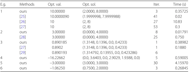
[image:11.595.117.481.593.732.2]

To verify the performance of the proposed algorithm, some numerical experiments are reported and compared with the known methods [19–25]. The algorithm is implemented by Matlab 2016a, and the tests are run in a microcomputer with Intel(R) Xeon(R) proces-sor of 2.4 GHz, 4 GB of RAM memory, under the Win10 operational system. We used linprog solver to solve all linear programming problems, and the convergent error is set toεin our procedure. For these test examples, the numerical results compared with the current algorithms are demonstrated in Tables1and2, where the following notations have

Table 1 Numerical comparisons for test Examples1–6

E.g. Methods Opt. val. Opt. sol. Iter. Time (s) 1 ours 10.00000 (2.0000, 8.0000) 3 0.35725

[25] 10.0000090 (1.9999998, 7.9999988) 41 0.02

[26] 10 (2, 8) 27 10.83

[27] 10 (2, 8) 53 0.3

2 ours 3.00000 (0.0000, 4.0000) 8 0.01791 [28] 3.00000 (0.0000, 4.0000) 25 0.750 3 ours 0.890185 (1.3148, 0.1396, 0.0, 0.4233) 1 0.38982

[27] 0.8902 (1.3148, 0.1396, 0.0, 0.4233) 1 0.1880 [29] 0.890193 (1.314792, 0.13955, 0.0, 0.423286) 6

(12)

[image:12.595.117.478.97.283.2]

Table 2 Numerical comparisons with Ref. [12,30] for Example7

Dimension Methods Opt. val. Iter. Time (s)

n= 5 [12] –25.0 141 10.11

[30] –25.0 12 0.0187

ours –25.0 1 0.01254

n= 10 [12] –100.0 283 21.86

[30] –100.0 31 0.3342

ours –100.0 7 0.25649

n= 20 [12] –400.0 651 47.00

[30] –400.0 86 5.9396

ours –400.0 15 2.73556

n= 30 [12] –900.0 965 106.33

[30] –900.0 204 44.8577

ours –900.0 18 11.25635

n= 50 [12] –2500.0 1891 304.30

ours –2500.0 21 17.35219

n= 80 ours –6400.0 37 40.45623

n= 100 ours –10,000.0 51 44.35865

n= 150 ours –22,500.0 66 112.99298

been used in column headers: Opt.Val.: optimal value; Opt.Sol.: optimal solution; Iter.: the number of iterations.

Example1 (Refs. [25–27])

⎧ ⎪ ⎪ ⎪ ⎪ ⎪ ⎪ ⎪ ⎪ ⎪ ⎪ ⎪ ⎪ ⎪ ⎪ ⎪ ⎪ ⎪ ⎪ ⎪ ⎪ ⎪ ⎪ ⎪ ⎨ ⎪ ⎪ ⎪ ⎪ ⎪ ⎪ ⎪ ⎪ ⎪ ⎪ ⎪ ⎪ ⎪ ⎪ ⎪ ⎪ ⎪ ⎪ ⎪ ⎪ ⎪ ⎪ ⎪ ⎩

min(y1+y2)(y1–y2+ 7)

s.t. 2y1+y2≤14,

y1+y2≤10,

– 4y1+y2≤0,

2y1+y2≥6,

y1+ 2y2≥6,

y1–y2≤3,

y1≤5,

y1+y2≥0,

y1–y2+ 7≥0.

Example2 (Ref. [28])

⎧ ⎪ ⎪ ⎪ ⎪ ⎪ ⎪ ⎪ ⎪ ⎪ ⎪ ⎪ ⎨ ⎪ ⎪ ⎪ ⎪ ⎪ ⎪ ⎪ ⎪ ⎪ ⎪ ⎪ ⎩

miny1+ (2y1– 3y2+ 13)(y1+y2– 1)

s.t. –y1+ 2y2≤8,

–y2≤–3,

y1+ 2y2≤12,

y1– 2y2≤–5,

(13)

Example3 (Refs. [27,29]) ⎧ ⎪ ⎪ ⎪ ⎪ ⎪ ⎪ ⎪ ⎪ ⎪ ⎪ ⎪ ⎪ ⎪ ⎪ ⎪ ⎪ ⎪ ⎪ ⎪ ⎪ ⎪ ⎪ ⎪ ⎪ ⎪ ⎪ ⎨ ⎪ ⎪ ⎪ ⎪ ⎪ ⎪ ⎪ ⎪ ⎪ ⎪ ⎪ ⎪ ⎪ ⎪ ⎪ ⎪ ⎪ ⎪ ⎪ ⎪ ⎪ ⎪ ⎪ ⎪ ⎪ ⎪ ⎩

min(0.813396y1+ 0.67440y2+ 0.305038y3+ 0.129742y4+ 0.217796)

×(0.224508y1+ 0.063458y2+ 0.932230y3+ 0.528736y4+ 0.091947)

s.t. 0.488509y1+ 0.063565y2+ 0.945686y3+ 0.210704y4≤3.562809,

–0.324014y1– 0.501754y2– 0.719204y3+ 0.099562y4≤–0.052215,

0.445225y1– 0.346896y2+ 0.637939y3– 0.257623y4≤0.427920,

–0.202821y1+ 0.647361y2+ 0.920135y3– 0.983091y4≤0.840950,

–0.886420y1– 0.802444y2– 0.305441y3– 0.180123y4≤–1.353686,

–0.515399y1– 0.424820y2+ 0.897498y3+ 0.187268y4≤2.137251,

–0.591515y1+ 0.060581y2– 0.427365y3+ 0.579388y4≤–0.290987,

0.423524y1+ 0.940496y2– 0.437944y3– 0.742941y4≤0.373620,

y1≥0,y2≥0,y3≥0,y4≥0.

Example4 ⎧ ⎪ ⎪ ⎪ ⎪ ⎪ ⎪ ⎪ ⎪ ⎪ ⎪ ⎪ ⎪ ⎪ ⎪ ⎨ ⎪ ⎪ ⎪ ⎪ ⎪ ⎪ ⎪ ⎪ ⎪ ⎪ ⎪ ⎪ ⎪ ⎪ ⎩

min6.5y1– 0.5y21–y2– 2y3– 3y4– 2y5–y6

s.t. y1+ 2y2+ 8y3+y4+ 3y5+ 5y6≤16,

–8y1– 4y2– 2y3+ 2y4+ 4y5–y6≤–1,

2y1+ 0.5y2+ 0.2y3– 3y4–y5– 4y6≤24,

0.2y1+ 2y2+ 0.1y3– 4y4+ 2y5+ 2y6≤12,

–0.1y1– 0.5y2+ 2y3+ 5y4– 5y5+ 3y6≤3,

0≤yi≤10,i= 1, 2, . . . , 6. Example5 ⎧ ⎪ ⎪ ⎪ ⎪ ⎪ ⎪ ⎪ ⎪ ⎪ ⎪ ⎪ ⎨ ⎪ ⎪ ⎪ ⎪ ⎪ ⎪ ⎪ ⎪ ⎪ ⎪ ⎪ ⎩

min2y1+ 3y2– 2y12– 2y22+ 2y1y2

s.t. –y1+y2≤1,

y1–y2≤1,

–y1+ 2y2≤3,

2y1–y2≤3,

0≤y1≤15, 0≤y2≤15.

Example6 ⎧ ⎪ ⎪ ⎨ ⎪ ⎪ ⎩

minyT_Qy₊_cT_y

s.t. Ay≤b, y∈Y0₌_{₀_≤_y

1≤2, 0≤y2≤2},

wherec= (2, 4)T_,_b_{= (1, 2, 4, 3, 1)}T_,_Q₌–1 2 2 –4

,A=

(14)

Example7 (Ref. [12])

⎧ ⎪ ⎪ ⎨ ⎪ ⎪ ⎩

min–n_i₌₁y2

i

s.t. j_i₌₁yi≤j,j= 1, 2, . . . ,n, yi≥0,i= 1, 2, . . . ,n.

Table2lists the numerical results of our algorithm, Gao’s algorithm [12], and Jiao’s algo-rithm [30] on Example7. By comparing the numerical results in Table2, we can conclude that our algorithm applied to Example7is superior to Gao’s algorithm [12] and Jiao’s al-gorithm [30] in terms of number of iterations and time.

Some randomly generated test examples with a large scale number of variables and con-straints are used to validate the robustness of the proposed algorithm. These randomly generated examples and their computational results are given as follows.

Example8

⎧ ⎪ ⎪ ⎨ ⎪ ⎪ ⎩

minyT_Qy₊_cT_y

s.t. Ay≤b,

y∈Y0₌_{_–10_≤_y

i≤10,i= 1, 2, . . . ,n},

whereQn×nis a real symmetric matrix, all the real elements ofQn×n,Am×n, andcn×1are

randomly generated in Interval [–2, 2], all the real elements ofbm×1are randomly

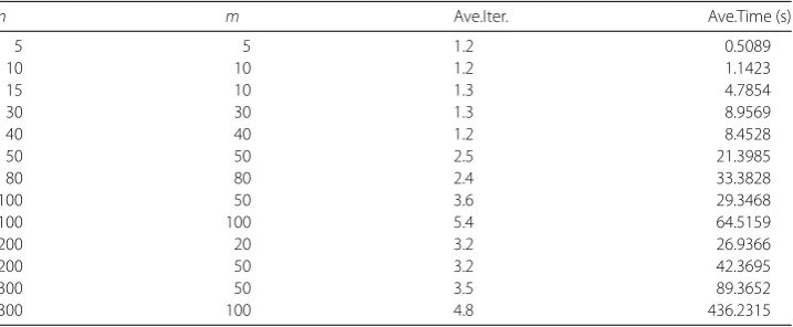
gener-ated in Interval [1, 10]. For Example8, we solved 10 diﬀerent random instances for each size and presented statistics of the results. The computational results are summarized in Table3, where the following notations have been used in column headers: Ave.Iter.: the average number of iterations; Ave.Time (s): the average CPU execution time for the algo-rithm in seconds;m: the number of constraints;n: the number of variables.

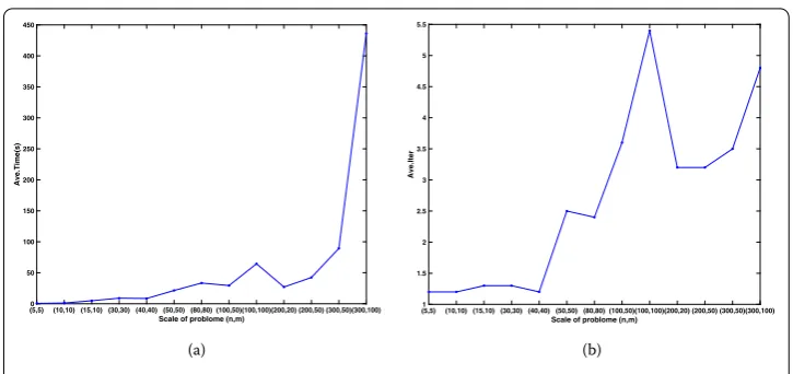
[image:14.595.119.478.584.732.2]

From Table3and Fig.1, it can be seen that, whenmandnare below 50, the algorithm can ﬁnd the global optimal solution in a short time and with lower iteration number. As the problem size becomes larger, the average number of iterations and the average CPU time of our algorithm are also increased, but they are not very sensitive to the problem size.

Table 3 Numerical results for Example8

n m Ave.Iter. Ave.Time (s)

5 5 1.2 0.5089

10 10 1.2 1.1423

15 10 1.3 4.7854

30 30 1.3 8.9569

40 40 1.2 8.4528

50 50 2.5 21.3985

80 80 2.4 33.3828

100 50 3.6 29.3468

100 100 5.4 64.5159

200 20 3.2 26.9366

200 50 3.2 42.3695

300 50 3.5 89.3652

(15)

[image:15.595.116.479.79.250.2]

(a) (b)

Figure 1The variation tendency of performance index with scale of Example8

From the experimental results in Table3, we can see that the proposed algorithm with the given convergent error can be used to globally solve the (NQP) with a large scale num-ber of constraints and variables. The results in Tables1–3show that our algorithm is both feasible and eﬃcient.

5 Concluding remarks

In this paper, we propose a new branch-and-bound algorithm for globally solving the non-convex quadratic programming problem. In this algorithm, we present a new linear re-laxation method, which can be used to derive the linear programs rere-laxation problem of the investigated problem (NPQ). To accelerate the computational speed of the proposed branch-and-bound algorithm, an interval deleting rule is used to reduce the investigated regions. By subsequently partitioning the initial region and solving a sequence of linear programs relaxation problems, the proposed algorithm is convergent to the global optima of the initial problem (NPQ). Finally, compared with some existent algorithms, numerical results show higher computational eﬃciency of the proposed algorithm.

Acknowledgements

The authors are grateful to the responsible editor and the anonymous referees for their valuable comments and suggestions, which have greatly improved the earlier version of this paper.

Funding

This work is supported by the National Natural Science Foundation of China (No. 61373174, No. 11501168, No. 11602184); the Science and Technology Key Project of Education Department of Henan Province (No. 16A110030).

Competing interests

The authors declare that they have no competing interests.

Authors’ contributions

All authors contributed equally to the manuscript, and they read and approved the ﬁnal manuscript.

Publisher’s Note

Springer Nature remains neutral with regard to jurisdictional claims in published maps and institutional aﬃliations.

Received: 15 April 2018 Accepted: 4 July 2018 References

(16)

2. Kedem, G., Watanabe, H.: Graph-optimization techniques for IC layout and compaction. IEEE Trans. Comput.-Aided Des. Integr. Circuits Syst.3(1), 12–20 (1984)

3. Lodwick, W.A.: Preprocessing nonlinear functional constraints with applications to the pooling problem. INFORMS J. Comput.4, 119–131 (1992)

4. Floudas, C.A., Visweswaran, V.: Primal-relaxed dual global optimization approach. J. Optim. Theory Appl.78(2), 187–225 (1993)

5. Li, Y., Kang, L., Garis, H.D., Kang, Z., Liu, P.: A robust algorithm for solving nonlinear programming problems. Int. J. Comput. Math.79(5), 523–536 (2002)

6. Shen, C., Xue, W., Pu, D.: A globally convergent trust region multidimensional ﬁlter SQP algorithm for nonlinear programming. Int. J. Comput. Math.86(12), 2201–2217 (2009)

7. Wang, H., Liu, F., Gu, C., Pu, D.: An infeasible active-set QP-free algorithm for general nonlinear programming. Int. J. Comput. Math.94(5), 884–901 (2016)

8. Vandenbussche, D., Nemhauser, G.L.: A branch-and-cut algorithm for nonconvex quadratic programs with box constraints. Math. Program.102(3), 559–575 (2005)

9. Burer, S., Vandenbussche, D.: Globally solving box-constrained nonconvex quadratic programs with semideﬁnite-based ﬁnite branch-and-bound. Comput. Optim. Appl.43(2), 181–195 (2009)

10. Cambini, R., Sodini, C.: Decomposition methods for solving nonconvex quadratic programs via branch and bound. J. Glob. Optim.33(3), 313–336 (2005)

11. Li, H.M., Zhang, K.C.: A decomposition algorithm for solving large-scale quadratic programming problems. Appl. Math. Comput.173(1), 394–403 (2006)

12. Gao, Y., Xue, H., Shen, P.: A new rectangle branch-and-reduce approach for solving nonconvex quadratic programming problems. Appl. Math. Comput.168(2), 1409–1418 (2005)

13. Burer, S., Vandenbussche, D.: A ﬁnite branch-and-bound algorithm for nonconvex quadratic programming via semideﬁnite relaxations. Math. Program.113(2), 259–282 (2008)

14. Al-Khayyal, F.A., Larsen, C., Voorhis, T.V.: A relaxation method for nonconvex quadratically constrained quadratic programs. J. Glob. Optim.6(3), 215–230 (1995)

15. Linderoth, J.: A simplicial branch-and-bound algorithm for solving quadratically constrained quadratic programs. Math. Program.103(2), 251–282 (2005)

16. Raber, U.: A simplicial branch-and-bound method for solving nonconvex all-quadratic programs. J. Glob. Optim. 13(4), 417–432 (1998)

17. Sherali, H.D., Adams, W.P.: A Reformulation-Linearization Technique for Solving Discrete and Continuous Nonconvex Problems, vol. 31. Springer, Berlin (1999)

18. Audet, C., Hansen, P., Jaumard, B., Savard, G.: A branch and cut algorithm for nonconvex quadratically constrained quadratic programming. Math. Program.87(1), 131–152 (2000)

19. Lu, C., Deng, Z., Jin, Q.: An eigenvalue decomposition based branch-and-bound algorithm for nonconvex quadratic programming problems with convex quadratic constraints. J. Glob. Optim.67(3), 475–493 (2017)

20. Gao, Y., Shang, Y., Zhang, L.: A branch and reduce approach for solving nonconvex quadratic programming problems with quadratic constraints. Oper. Res. Trans.9(2), 9–20 (2005)

21. Qu, S.J., Zhang, K.C., Ji, Y.: A global optimization algorithm using parametric linearization relaxation. Appl. Math. Comput.186(1), 763–771 (2007)

22. Shen, P., Duan, Y., Ma, Y.: A robust solution approach for nonconvex quadratic programs with additional multiplicative constraints. Appl. Math. Comput.201(1–2), 514–526 (2008)

23. Shen, P., Liu, L.: A global optimization approach for quadratic programs with nonconvex quadratic constraints. Chin. J. Eng. Math.25(5), 923–926 (2008)

24. Shen, P., Wang, C.: Linear decomposition approach for a class of nonconvex programming problems. J. Inequal. Appl. 2017(1), 74 (2017)

25. Chen, Y., Jiao, H.: A nonisolated optimal solution of general linear multiplicative programming problems. Comput. Oper. Res.36(9), 2573–2579 (2009)

26. Gao, Y., Wu, G., Ma, W.: A new global optimization approach for convex multiplicative programming. Appl. Math. Comput.216(4), 1206–1218 (2010)

27. Wang, C.F., Liu, S.Y., Shen, P.P.: Global minimization of a generalized linear multiplicative programming. Appl. Math. Model.36(6), 2446–2451 (2012)

28. Jiao, H.W., Liu, S.Y., Zhao, Y.F.: Eﬀective algorithm for solving the generalized linear multiplicative problem with generalized polynomial constraints. Appl. Math. Model.39(23–24), 7568–7582 (2015)

29. Thoai, N.V.: A global optimization approach for solving the convex multiplicative programming problem. J. Glob. Optim.1(4), 341–357 (1991)