On complexity of a new Mehrotra type interior point algorithm for \(P {*}(\kappa )\) linear complementarity problems

(1)

R E S E A R C H

Open Access

On complexity of a new Mehrotra-type

interior point algorithm for

P

_∗

(

κ

)

linear

complementarity problems

Yiyuan Zhou

1,2*

_{, Mingwang Zhang}

1,2

_{and Zhengwei Huang}

3

*_{Correspondence:}_{zyy@ctgu.edu.cn}

1_{College of Science, China Three}

Gorges University, Yichang, P.R. China

2_{Three Gorges Mathematical}

Research Center, China Three Gorges University, Yichang, P.R. China

Full list of author information is available at the end of the article

Abstract

In this paper, a variant of Mehrotra-type predictor–corrector algorithm is proposed for P_∗(

κ

) linear complementarity problems. In this algorithm, a safeguard step is used to avoid small step sizes and a new corrector direction is adopted. The algorithm has polynomial iteration complexity and the iteration bound is

O((14

κ

+ 11)√(1 + 4

κ

)(1 + 2

κ

)nlog(x0)_εTs0). Some numerical results are reported as well.

MSC: 90C51; 90C33

Keywords: Interior point algorithm;P_∗(

κ

) linear complementarity problem; Mehrotra-type algorithm; Polynomial complexity

1 Introduction

AP∗(κ) linear complementarity problem (LCP) is to ﬁnd vectorsx∈Rn_and_s_∈_Rn_such that

Mx+q=s,

xTs= 0,

x,s≥0,

(1)

whereM∈Rn×n_{is a}_P

∗(κ) matrix andq∈Rn.

LCPs are closely associated with linear programming and quadratic programming. It is well known that a diﬀerentiable convex quadratic programming can be formulated as a monotone LCP by exploiting the ﬁrst-order optimality conditions, and vice versa [1]. Transportation planning and game theory also have a close connection with LCPs [2,3].

Interior point algorithms for LCPs have been widely studied in the last few decades [4]. In 1991, Kojima et al. [5] extended all the previously known results toP∗(κ) LCPs and uniﬁed the theory of LCPs from the view point of interior point methods. Since then, many interior point algorithms for linear programming have been extended toP∗(κ) LCPs. Illés

and Nagy [6], and Miao [7] studied the Mizuno-Todd-Ye type interior point algorithms onP∗(κ) LCPs. Cho [8], and Cho and Kim [9] proposed two interior point polynomial

algorithms based on kernel functions forP∗(κ) LCPs. Using a new updating strategy of

(2)

the centering parameter, Liu et al. [10] extended two Mehrotra-type predictor–corrector algorithms to suﬃcient LCPs.

Predictor–corrector algorithms are practical interior point methods for linear program-ming, quadratic programming and LCPs, variants of which have become backbones of several optimization software packages [11, 12]. Mehrotra [13] proposed a predictor– corrector algorithm for linear programming, in which the coefficient matrices in both predictor steps and corrector steps are the same, and it needs less computational efforts than other methods. After that, several variants of this algorithm have been studied. Jarre and Wechs [14] studied a new primal–dual interior point method in which the search di-rections are based on corrector didi-rections of Mehrotra-type algorithm. Zhang and Zhang [15] presented a second order Mehrotra-type predictor–corrector algorithm without up-dating the central path. Salahi et al. [16] found that in a variant of Mehrotra’s algorithm, in order to keep iterates in a large neighborhood of the central path, some steps are very small. To avoid small or zero steps, Salahi et al. introduced some safeguards in the cor-rector steps [16] and a new criterion on predictor step sizes [17], moreover, they proved that the two algorithms have polynomial complexity and practical efficiency. Infeasible versions of Mehrotra-type algorithms are studied by Liu et al. [18], and Yang et al. [19].

In this paper, a new variant of Mehrotra-type predictor–corrector algorithm is proposed forP∗(κ) LCPs. In this algorithm, the corrector step is diﬀerent from other Mehrotra-type predictor–corrector algorithms [16, 17]. If (x, s) is the search direction of a P∗(κ) LCP, thenxTs= 0, whilexTs= 0 if (x,s) is the search direction of

lin-ear programming. So the analysis is diﬀerent from that in linlin-ear programming. If an it-eration (x,s) takes a step along the corrector direction (x,s), the parameterμg(α) = (1 –α)μg+αμ–αα2ax

aT_sa

n +α2 xT_s

n , whereαais the predictor step size and (xa,sa) is the predictor search direction. In order to reduce the dual gapxT_s_{, the corrector step size} αshould be chosen such thatμg(α)≤μg, that is to say,αshould have an upper bound. Ifα is larger than a given threshold, then the threshold is chosen as the corrector step size. The iteration complexity of the new algorithm isO((14κ+ 11)√(1 + 4κ)(1 + 2κ)nlog(x0)_εTs0), which is analogous to that of linear programming.

This paper is organized as follows. In Sect.2, a new Mehrotra-type predictor–corrector algorithm forP∗(κ) LCPs is introduced. In Sect.3, the polynomial iteration complexity is provided. Some illustrative numerical results are reported in Sect.4. Finally, some con-cluding remarks are given in Sect.5.

We use the following notations throughout the paper:·denotes the 2-norm of vectors, eis then-dimensional vector of ones. For any twon-dimensional vectorsxands,xsis the componentwise product of the two vectors. We also use the following notations.

I={1, 2, . . . ,n}, I+=

i∈I|xa_isa_i ≥0, I–=

i∈I|xa_isa_i < 0,

F+=

(x,s)∈Rn×Rn|s=Mx+q, (x,s)≥0,

F++=

(x,s)∈Rn×Rn|s=Mx+q, (x,s) > 0.

2 Mehrotra-type predictor–corrector algorithm

A matrixM∈Rn×n_{is a}_P

∗(κ) matrix [5] if

(1 + 4κ) j∈J+

xj(Mx)j+

j∈J–

(3)

or

xTMx≥–4κ j∈J+

xj(Mx)j, ∀x∈Rn, (3)

whereκ≥0,J+={j|j∈I,xj(Mx)j≥0}, andJ–={j|j∈I,xj(Mx)j< 0}.

Noting that the positive semi-deﬁnite matrix is aP∗(0) matrix, thus the class ofP∗(κ) matrices includes the class of positive semi-deﬁnite matrices. Other properties ofP∗(κ)

matrices can be found in [5].

Without loss of generality [5], we assume that theP∗(κ) LCP (1) satisﬁes the interior point condition, that is, there exists a point (x0_,_s0_{) such that}

s0₌_Mx0₊_q_, _x0_{> 0,}_s0_{> 0.}

To ﬁnd an approximate solution of (1), the following parameterized system is estab-lished:

Mx+q=s,

xs=μe,

x,s≥0,

(4)

whereμ> 0.

If theP∗(κ) LCP (1) satisﬁes the interior point condition, then the system (4) has a unique solution for anyμ> 0. For a givenμ, the solution, denoted by (x(μ),s(μ)), is called aμ -center of (1). The set of allμ-centers gives the central path of (1). A primal–dual interior point algorithm follows the central path{(x(μ),s(μ))|μ> 0}approximately and approaches the solution of (1) asμgoes to zero.

Most interior point algorithms work in the neighborhoodN–

∞(γ) deﬁned by

N_∞–(γ) =(x,s)∈F++|xisi≥γ μg,∀i∈I

,

whereγ ∈(0, 1) is a constant independent ofnandμg=x

T_s

n .

Now, based on [16], a new variant of Mehrotra-type predictor–corrector algorithm for P∗(κ) LCPs will be described.

The predictor search direction (xa,sa) is determined by the following equations:

Mxa=sa,

sxa+xsa= –xs.

(5)

The predictor step sizeαais deﬁned by

αa=max

α|0≤x+αaxa,s+αasa

, 0 <α≤1. (6)

(4)

(x,s) by solving the following system:

Mx=s,

sx+xs=μe–xs–α2_axasa,

(7)

where

μ=

ga g

2

ga

n (8)

withga= (x+αaxa)T(s+αasa) andg=xTs. The second equation of (7) is diﬀerent from that in [16], where it issx+xs=μe–xs–xa_sa_.

The next iterate is denoted by

x(α) =x+αx,s(α) =s+αs,

whereαis the corrector step size deﬁned by

α=maxα|x(α),s(α)∈N_∞–(γ), 0 <α≤1. (9)

In order to avoid small steps, we combine Mehrotra’s updating strategy of the center-ing parameter with a safeguard step at each iteration. The new Mehrotra-type predictor– corrector algorithm forP∗(κ) LCPs is stated as Algorithm1.

Algorithm 1Mehrotra-type predictor–corrector algorithm forP∗(κ) LCPs

Input:

A proximity parameterγ∈(0,₄_κ1₊₅); an accuracy parameterε> 0; a starting point (x0_,_s0₎_∈_N–

∞(γ).

whilexTs≥εdo

begin(Predictor Step)

Solve (5) and compute the predictor step sizeαaby (6).

end

begin(Corrector Step)

Ifαa≥0.3, then solve (7) withμ= (g_ga)2g_na and compute the corrector step sizeαby (9).

end

Ifαa< 0.3 orα<₁₆7γ_pn, wherep=11+14₁₆ κ

√

(1 + 4κ)(2 + 4κ), then solve (7) withμ=_1–γ_γμgand compute the corrector step sizeα.

end

Ifthe corrector step sizeα>α1, then letα=α1,

whereα1=1–2γ–(1–γ)κα

2 a

2q(1–γ) andq= 14κ+11

16 .

end

Set (x,s) = (x(α),s(α)).

(5)

3 Complexity analysis

The polynomial complexity of Algorithm1will be discussed in this section. Firstly, we present three important lemmas which will be used in convergence analysis.

Lemma 1([16]) Let(xa,sa)be the solution of(5).Then

xa_isa_i ≤1

4xisi, ∀i∈I+,

–xa_isa_i ≤ 1 αa

1

αa – 1

xisi, ∀i∈I–,

i∈I+

xa_isa_i ≤x T_s

4 .

Lemma 2 Let M be a P∗(κ)matrix and(xa,sa)be the solution of(5).Then

i∈I–

xa_isa_i ≤4κ+ 1

4 x

T_s_,

–κxTs≤xaTsa≤x T_s

4 .

Proof SinceMis aP∗(κ) matrix, we have

0≥

i∈I–

xa_isa_i ≥–(4κ+ 1) i∈I+

xa_isa_i ≥–4κ+ 1

4 x

T_s_,

where the last inequality is due to the third conclusion of Lemma1. Furthermore, from (3), we get

xaTsa≥–4κ i∈I+

xa_isa_i ≥–4κx T_s

4 = –κx T_s_.

This completes the proof.

Lemma 3 Let M be a P∗(κ)matrix and(x,s)be the solution of(7)withμ> 0.Then

xs ≤

1 4+κ

1 2+κ

μ(xs)–12 _{– (}_xs₎12 _–_α2

a(xs)–

1

2_xa_sa2_,

i∈I+

xisi≤ 1 4μ(xs)

–1₂ _{– (}_xs₎1₂ _–_α2

a(xs)–

1

2_xa_sa2_.

Proof The proof is similar to that of Lemma 8 in [6], and it is omitted.

According to (8) and Lemma2, it can be found that

ga g

2

ga n =

[(1 –αa)xTs+α2a(xa)Tsa]3 n(xT_s₎2

(6)

=

1 –αa+ 1 4α

2

a 3

μg

≤

1 –3

4αa 3

μg. (10)

Consequently, _μμ

g≤(1 –

3

4αa)3ifμ= (

ga

g )2 ga

n.

The following theorem shows that the predictor step size has a lower bound.

Theorem 4 Let the current iterate(x,s)∈N_∞–(γ), (xa,sa)be the solution of(5)andαa be the predictor step size.Then

αa≥

γ

(4κ+ 1)n.

Proof According to (5), we get

xi+αxai

si+αsai

= (1 –α)xisi+α2xaisai.

Following from Lemma2, we havexa_isa_i ≥0 ifi∈I+andxaisai ≥–4 κ+1

4 xTsifi∈I–.

Therefore, for alli∈I,

xa_isa_i ≥–4κ+ 1

4 x

T_s_.

Noting that (x,s)∈N_∞–(γ) impliesxisi≥γ μg, we have

(1 –α)xisi+α2xaisai ≥(1 –α)γ xT_s

n – 4κ+ 1

4 α

2_xT_s_.

Thus, to show (x+αxa_,_s₊_α_sa₎_∈_F

+, one has to prove the following inequality:

(4κ+ 1)nα2+ 4γ α– 4γ ≤0. (11)

Clearly, inequality (11) is true if

0≤α≤2

γ2_{+ (4}_κ_{+ 1)}_n_γ _{– 2}_γ

(4κ+ 1)n .

Therefore, the predictor step sizeαasatisﬁes

αa≥

2γ2_{+ (4}_κ_{+ 1)}_n_γ _{– 2}_γ

(4κ+ 1)n .

Since 0 <₍₄_κγ₊₁₎_n<₄_κ1₊₁₄_κ1₊₅1_n<1₂, it can be found that

2γ2_{+ (4}_κ_{+ 1)}_n_γ _{– 2}_γ

(4κ+ 1)n =

2

1 +1 + (4κ+ 1)_γn ≥

γ

(4κ+ 1)n.

(7)

In what follows, the lower bound ofαais used as the default predictor step size with the notation

αa=

γ

(4κ+ 1)n. (12)

Lemma 5 If(x,s)∈N–

∞(γ),and(x,s)is the solution of(7)withμ≥0,then

xs≤ω

1 4+κ

1 2+κ

and

xTs≤1 4ω,

whereω=n_{γ μ}μ2

g– 2nμ+

nμα2a(4κ+1)

2γ +

αa4+8α2a+4α2a(4κ+1)(1–αa)+16 16 nμg.

Proof From Lemma3, we have

xs ≤

1 4+κ

1 2+κ

μ(xs)–12 _{– (}_xs₎12 _–_α2

a(xs)–

1

2_xa_sa2

and

xTs≤1 4μ(xs)

–1₂ _{– (}_xs₎1₂ _–_α2

a(xs)–

1

2_xa_sa2_,

where

μ(xs)–12 _{– (}_xs₎12_–_α2

a(xs)–

1

2_xa_sa2

=μ2 i∈I

1 xisi

+

i∈I

xisi– 2nμ+αa4

i∈I (xa

isai)2 xisi

– 2μα2_a i∈I

xa isai xisi

+ 2α_a2 i∈I

xa_isa_i.

Sincexisi≥γ μg for alli∈I, we have

μ2 i∈I

1 xisi

≤ nμ2 γ μg .

From Lemma1and Lemma2, it follows that

i∈I

(xa_isa_i)2

xisi

=

i∈I+

(xa_isa_i)2

xisi

+

i∈I–

(xa_isa_i)2

xisi

≤

i∈I+

(xisi

4 ) 2

xisi

+

i∈I–

–xa isai xisi

(8)

≤xTs

16 + 1 –αa

α2

a

i∈I–

xa_isa_i

≤nμg 16 +

(1 –αa)(4κ+ 1)nμg 4α2

a

.

Since (x,s)∈N–

∞(γ) andi∈I–|x

a

isai| ≤4κ4+1xTs, we obtain

–2μ

i∈I xa

isai xisi ≤

2μ

i∈I–

|xa isai| xisi ≤

2μ γ μg

i∈I–

xa_isa_i ≤nμ(4κ+ 1)

2γ .

As_i_∈_I₊xa isai ≤x

T_s

4 , we get

2

i∈I

xa_isa_i ≤2 i∈I+

xa_isa_i ≤nμg 2 .

Combining the above inequalities yields the result of this lemma.

Corollary 6 If(x,s)∈N_∞–(γ),γ ∈(0,₄_κ1₊₅),and(x,s)is the solution of(7)withμ=

γ

1–γμg,then

xs ≤pnμg, xTs≤qnμg,

where p=14κ+11 16

√

(1 + 4κ)(2 + 4κ)and q=14κ+11 16 .

Proof Since 0 <γ<₄_κ1₊₅≤₅1, we have _(1–γ_γ₎2 ≤₁₆5 and

α_a2(4κ+1)–4γ 2(1–γ) ≤

5α2_a(4κ+1) 8 .

Ifμ=_1–γ_γμg, then

ω=

γ

(1 –γ)2 +

α_a2(4κ+ 1) – 4γ

2(1 –γ) +

α4_a+ 8α_a2+ 4α2_a(4κ+ 1)(1 –αa) + 16 16

nμg

≤

5 16+

5α_a2(4κ+ 1)

8 +

α_a4+ 8α2_a+ 4α_a2(4κ+ 1)(1 –αa) + 16 16

nμg

≤

5 16+

5(4κ+ 1)

8 +

1 + 8 + 4(4κ+ 1) + 16 16

nμg=

56κ+ 44 16 nμg,

where the second inequality follows from 0 <αa≤1. From Lemma5, it follows that

xs ≤ω

1 4+κ

1 2+κ

≤pnμg.

Similarly, the second result can easily be veriﬁed.

For simplicity, the following notation is used in the rest of this paper:

t=max

i∈I+

xa isai xisi

.

(9)

Theorem 7 Let(x,s)∈N–

∞(γ), (x,s)be the solution of(7)withμ=1–γγμgandαbe the corrector step size.Then

α≥ 7γ

16pn.

Proof The corrector step size is the maximumαsuch thatα∈(0, 1] and

xi(α)si(α)≥γ μg(α), ∀i∈I.

After a simple computation, we get

xi(α)si(α) =xisi+α

μ–xisi–αa2xaisai

+α2xisi

≥1 –α–αtα_a2xisi+αμ–α2pnμg,

where the inequality is due toxa

isai ≤txisi andxs ≤pnμg. Clearly, 1 +tαa2≤ 1 +1₄α_a2. Thus, for 0≤α≤ 1

1+1₄α2a, we have

xi(α)si(α)≥

1 –α–αtα_a2γ μg+αμ–α2pnμg.

Applying Lemma2and Corollary6yields

μg(α) =

(x+αx)T₍_s₊_α_s₎ n

= (1 –α)μg+αμ–ααa2

xaT_sa

n +α

2xTs

n

≤(1 –α)μg+αμ+ααa2κμg+α2qμg. (13)

To provexi(α)si(α)≥γ μg(α), one has to show that

1 –α–αtα_a2γ μg+αμ–α2pnμg≥γ

(1 –α)μg+αμ+αα2aκμg+α2qμg

.

Ifμ=_1–γ_γμg, then the above inequality is equivalent to

γ –γ κα_a2–tγ α_a2≥α(pn+qγ). (14)

Sinceαa=

γ

(4κ+1)n,γ < 1 andt≤

1

4, we have

γ –γ κα_a2–tγ α_a2≥γ– 4κγ

2₊_γ2

4n(4κ+ 1)≥γ –

4κγ+γ

4n(4κ+ 1)≥ 7 8γ.

Noting thatpn>qγ, then inequality (14) is true if 0≤α≤₁₆7γ_pn. We can conclude that the corrector step sizeαsatisﬁes

α≥min

1 1 +1

4α2a , 7γ

16pn

= 7γ

(10)

In Algorithm1, the corrector step sizeαhas an upper boundα1, that is,

α≤α1=

1 – 2γ – (1 –γ)κα2

a

2q(1 –γ) . (15)

The next theorem means that the upper bound is well deﬁned.

Theorem 8 Let αa be the default predictor step size and γ ∈(0,₄κ1+5). Then 7γ 16pn <

1–2γ–(1–γ)καa2

2q(1–γ) < 1.

Proof Sinceq=14κ₁₆+11>₂1, it is clear that1–2γ–(1–γ)καa2

2q(1–γ) < 1. Asn≥2 andp>q> 1

2, we have

7γ

16pn≤ 7γ

16.

According to (12), one hasκα_a2=_n₍₄κγ_κ₊₁₎≤γ₈, thus

1 – 2γ – (1 –γ)κα_a2

1 –γ ≥

1 – 2γ– (1 –γ)γ₈

1 –γ = 2 +

1

γ– 1–

γ

8.

Fromγ <₄_κ1₊₅≤1₅, it follows that

2 + 1

γ– 1–

γ

8 > 7γ

16.

Therefore

1 – 2γ – (1 –γ)κα_a2

2q(1 –γ) > 7γ

16pn,

which completes the proof.

In the following theorem, we obtain an upper bound of the iteration number.

Theorem 9 Algorithm1stops after at most

O

(14κ+ 11)(1 + 4κ)(1 + 2κ)nlog(x

0₎T_s0

ε

iterations with a solution for which xTs≤ε.

Proof Ifαa≥0.3 andα≥₁₆7γ_pn, then Algorithm1adopts Mehrotra’s strategy in the cor-rector step, i.e.,μ= (ga

g)2 ga

n. Based on (13), we have

μg(α)≤

1 –

1 –κα_a2–qα– μ

μg

α

μg

≤

1 –

1 –κα_a2–q1 – 2γ– (1 –γ)κα

2

a 2q(1 –γ) –

1 –3

4αa

3

α

μg

≤

1 –

1 – 0.0125 – 1 – 2γ 2(1 –γ)– 0.47

α

(11)

≤

1 – γ

2(1 –γ)α

μg

≤

1 – 7γ

2

32pn(1 –γ)

μg,

where the second inequality follows from (10) and (15), the third inequality is due toκα_a2≤

0.025 and 1 –3 4αa≤

31

40, and the fourth inequality comes from 1 – 0.0125 – 0.47≥ 1 2.

Ifαa< 0.3 orα<₁₆7γ_pn, then Algorithm1adopts the safeguard strategy in the corrector

step, that is,μ=_1–γ_γμg. In this case, from ₁₆7γ_pn≤α≤1–2

γ–(1–γ)κα2_a 2q(1–γ) , we get

μg(α)≤

1 –

1 –κα_a2–qα– μ

μg α μg ≤ 1 –

1 –κα_a2–q1 – 2γ– (1 –γ)κα

2

a 2q(1 –γ) –

γ

1 –γ

α μg = 1 –

1 – 2γ

2(1 –γ)–

κα2 a 2 α μg ≤

1 – (39 – 79γ)7γ 1280pn(1 –γ)

μg,

where the last inequality follows fromκα2

a≤0.025 andα≥

7γ

16pn. This completes the proof

by Theorem 3.2 of [1].

4 Numerical results

In this section, some numerical results are reported. The results are obtained by using MATLAB R2014a.

The algorithm presented in this paper is compared with a Mizuno–Todd–Ye (MTY) type predictor–corrector algorithm [6], Cho’s algorithm [8] and an interior point algorithm based on the classical kernel functionϕ(t) =t2–1

2 –logt(IPMCKF) [20]. We consider the

following two problems.

Problem 1([21])

M=

0 1

–2 0

, q=

2 3

, x0=

0.4 0.45

, s0=

2.45

2.2

.

Problem 2([22])

M= ⎛ ⎜ ⎜ ⎜ ⎜ ⎜ ⎜ ⎜ ⎝

1 2 2 · · · 2 2 5 6 · · · 6 2 6 9 · · · 10

..

. ... ... ... ... 2 6 10 · · · 4n– 3

⎞ ⎟ ⎟ ⎟ ⎟ ⎟ ⎟ ⎟ ⎠

, q=

⎛ ⎜ ⎜ ⎜ ⎜ ⎜ ⎜ ⎜ ⎝ –1 –1 –1 .. . –1 ⎞ ⎟ ⎟ ⎟ ⎟ ⎟ ⎟ ⎟ ⎠

, x0=

⎛ ⎜ ⎜ ⎜ ⎜ ⎜ ⎜ ⎜ ⎝ 1 1 1 .. . 1 ⎞ ⎟ ⎟ ⎟ ⎟ ⎟ ⎟ ⎟ ⎠ .

Problem1is aP∗(1₄) LCP, and Problem2is aP∗(0) LCP. We solve the two problems by

(12)

Table 1 The iteration numbers of Problem1

Algorithm1 MTY Cho’s IPMCKF

[image:12.595.219.375.155.254.2]

4 55 19 24

Table 2 The iteration numbers of Problem2

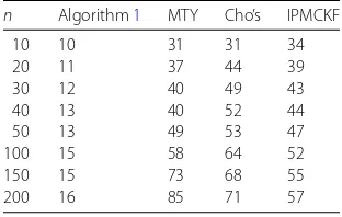
n Algorithm1 MTY Cho’s IPMCKF

10 10 31 31 34

20 11 37 44 39

30 12 40 49 43

40 13 40 52 44

50 13 49 53 47

100 15 58 64 52

150 15 73 68 55

200 16 85 71 57

Table1shows the iteration numbers of Algorithm1, MTY algorithm, Cho’s algorithm and IPMCKF algorithm for Problem1. From the results we conclude that Algorithm1

reduced the iteration numbers.

Table 2 gives the iteration numbers of the four algorithms for Problem2 with n∈

{10, 20, 30, 40, 50, 100, 150, 200}. The numerical results illustrate that Algorithm1has the least iteration numbers. Since the safeguard step helps Algorithm1to avoid small steps, Algorithm1is eﬃcient.

5 Concluding remarks

In this paper, a Mehrotra-type predictor–corrector algorithm forP∗(κ) LCPs is studied. SinceP∗(κ) LCPs are the generalization of linear programming, the search directionsx

andsare not orthogonal, therefore the analysis is diﬀerent from that in linear program-ming. The iteration bound of our algorithm isO((14κ+ 11)√(1 + 4κ)(1 + 2κ)nlog(x0)_εTs0). Numerical results show that this algorithm is eﬃcient.

Funding

This work was supported by the National Natural Science Foundation of China (71471102, 71561022 and 71771025).

Competing interests

The authors declare that they have no competing interests.

Authors’ contributions

All authors contributed equally to this work. All authors read and approved the ﬁnal manuscript.

Author details

1_{College of Science, China Three Gorges University, Yichang, P.R. China.}2_{Three Gorges Mathematical Research Center,} China Three Gorges University, Yichang, P.R. China.3_{College of Economics and Management, China Three Gorges} University, Yichang, P.R. China.

Publisher’s Note

Springer Nature remains neutral with regard to jurisdictional claims in published maps and institutional aﬃliations.

Received: 7 August 2018 Accepted: 1 January 2019

References

1. Wright, S.J.: Primal–Dual Interior-Point Methods. Society for Industrial and Applied Mathematics, Philadelphia (1997) 2. Billups, S.C., Murty, K.G.: Complementarity problems. J. Comput. Appl. Math.124(1), 303–318 (2000)

3. Cottle, R.W., Pang, J.S., Stone, R.E.: The Linear Complementarity Problem. Academic Press, New York (1992) 4. Roos, C., Terlaky, T., Vial, J.P.: Interior Point Methods for Linear Optimization. Springer, Boston (2006) 5. Kojima, M., Megiddo, N., Noma, T., Yoshise, A.: A Uniﬁed Approach to Interior Point Algorithms for Linear

(13)

6. Illes, T., Nagy, M.: A Mizuno–Todd–Ye type predictor–corrector algorithm for suﬃcient linear complementarity problems. Eur. J. Oper. Res.181(3), 1097–1111 (2007)

7. Miao, J.: A quadratically convergentO((1 +κ)√nL)-iteration algorithm for theP_∗(κ)-matrix linear complementarity problem. Math. Program.69(1), 355–368 (1995)

8. Cho, G.M.: A new large-update interior point algorithm forP_∗(κ) linear complementarity problems. J. Comput. Appl. Math.216(1), 265–278 (2008)

9. Cho, G.M., Kim, M.K.: A new large-update interior point algorithm forP∗(κ) LCPs based on kernel functions. Appl. Math. Comput.182(2), 1169–1183 (2006)

10. Liu, H., Liu, X., Liu, C.: Mehrotra-type predictor–corrector algorithms for suﬃcient linear complementarity problem. Appl. Numer. Math.62(12), 1685–1700 (2012)

11. Czyzyk, J., Mehrotra, S., Wagner, M., Wright, S.: Pcx: an interior-point code for linear programming. Optim. Methods Softw.11(1–4), 397–430 (1999)

12. Zhang, Y.: Solving large-scale linear programs by interior-point methods under the Matlab environment. Optim. Methods Softw.10(1), 1–31 (1998)

13. Mehrotra, S.: On ﬁnding a vertex solution using interior point methods. Linear Algebra Appl.152(91), 233–253 (1991) 14. Jarre, F., Wechs, M.: Extending Mehrotra’s corrector for linear programs. Adv. Model. Optim.1(2), 38–60 (1999) 15. Zhang, Y., Zhang, D.: On polynomiality of the Mehrotra-type predictor–corrector interior-point algorithms. Math.

Program.68(1), 303–318 (1995)

16. Salahi, M., Peng, J., Terlaky, T.: On Mehrotra-type predictor–corrector algorithms. SIAM J. Optim.18(4), 1377–1397 (2007)

17. Salahi, M., Terlaky, T.: Mehrotra-type predictor–corrector algorithm revisited. Optim. Methods Softw.23(2), 259–273 (2008)

18. Liu, X., Liu, H., Wang, W.: Polynomial convergence of Mehrotra-type predictor–corrector algorithm for the Cartesian

P∗(κ)-LCP over symmetric cones. Optimization64(4), 815–837 (2015)

19. Yang, X., Liu, H., Dong, X.: Polynomial convergence of Mehrotra-type prediction-corrector infeasible-IPM for symmetric optimization based on the commutative class directions. Appl. Math. Comput.230(2), 616–628 (2014) 20. Lesaja, C., Roos, C.: Uniﬁed analysis of kernel-based interior-point methods forP∗(κ)-linear complementarity

problems. SIAM J. Optim.20(6), 3014–3039 (2010)

21. Lee, Y.-H., Cho, Y.-Y., Cho, G.-M.: Interior-point algorithms forP∗(κ) LCP based on a new class of kernel functions. J. Glob. Optim.58, 137–149 (2014)