Globally Convergent Algorithms for Maximum a Posteriori Transmission Tomography

(1)

Globally Convergent Algorithms

for Maximum

a

Posteriori

Transmission Tomography

Kenneth

Lange

and

Jeffrey

A.

Fessler, Member,

IEEE

Absh-uct- This paper reviews and compares three maximum likelihood algorithms for transmission tomography. One of these algorithms is the EM algorithm, one is based on a convexity argument devised by De Pierro in the context of emission tomog- raphy, and one is an ad hoc gradient algorithm. The algorithms enjoy desirable local and global convergence properties and combine gracefully with Bayesian smoothing priors. Preliminary numerical testing of the algorithms on simulated data suggest that the convex algorithm and the ad hoc gradient algorithm are computationally superior to the EM algorithm. This superiority stems from the larger number of exponentiations required by the EM algorithm. The convex and gradient algorithms are well adapted to parallel computing.

I. INTRODUCTION

HE value of the EM algorithm in emission tomography is

T

now well established [22], [17], [24]. Not as widely ap- preciated is the potential of the EM algorithm in transmission tomography [17]. This paper reviews the EM algorithm for transmission tomography and compares it to two algorithms recently introduced by Lange et al. 1161 and Lange 1121.

The traditional method of image reconstruction in transmission tomography relies on Fourier analysis and the Radon transform [lo]. An alternative to this deterministic reconstruction method is to pose an explicitly stochastic model that permits parameter estimation by maximum likelihood [17]. In this context the EM algorithm provides an easily implemented method for searching the likelihood surface. This does not mean that the EM or competing stochastic algorithms can match Fourier methods in computational speed. But the increased realism possible with a stochastic model does promise better image reconstruction with lower patient radiation dose.

The object of transmission tomography is to reconstruct the local attenuation properties of the object being imaged. Attenuation is roughly to be equated with density. In an imaging experiment, X-rays or y-rays are beamed from an external source through the imaged object. These high energy photons can be stopped or deflected by the object, or they can be detected by a device on the opposite side of the object. Only a fraction of the photons successfully travel from source to

Manuscript received September 14, 1994; revised December 6, 1994. K. Lange was supported in part by USPHS Grant CA-16042. J. A. Fessler was supported in part by USPHS Grant CA-60711 and DOE Grant DE-FG02- 87ER60561. The associate editor coordinating the review of this paper and approving it for publication was Prof. Ken D. Sauer.

K. Lange is with the Department of Biostatistics, School of Public Health, University of Michigan, Ann Arbor, MI 48109-2029 USA.

J. A. Fessler is with the Division of Nuclear Medicine, Department of Internal Medicine, University of Michigan, Ann Arbor, MI 48109-0552 USA.

IEEE Log Number 9413846.

detector along a given flight path (projection). The probability of a photon escaping attenuation along a projection is given by exponentiating the negative of the line integral of the attenuation density along the projection. In deterministic reconstruction, these line integrals are mathematically massaged to given the final image. No account is taken of the fact that the observed data actually consist of photon counts.

The stochastic model depends on dividing the object of interest into small nonoverlapping regions of constant attenuation called pixels. Typically the pixels are squares. To each pixel is assigned an attenuation parameter. In the absence of the intervening object, the number of photons generated and ultimately detected along a projection follows a Poisson distribution. Attenuation randomly thins these photons. Since thinning a Poisson process yields a Poisson process, the number of photons detected also follows a Poisson distribution. The detected photon counts constitute the observed data for stochastic reconstruction.

The remainder of this paper builds on the above verbal model of transmission tomography. Section

I1

motivates three competing algorithms for maximum likelihood estimation of the attenuation parameters. Local convergence of the algorithms is examined under the simplifying assumption that the maximum point is interior to the feasible region. Section 111

outlines how the algorithms can be amended to incorporate Bayesian smoothing parameters. Section IV proves that two of the algorithms are globally convergent. Section V compares the numerical performance of the algorithms on simulated data. The concluding discussion in Section VI draws some preliminary conclusions about the numerical efficiency of the algorithms and suggests topics for further research.

11. ALGORITHMS FOR TRANSMISSION TOMOGRAPHY

The parameters of interest in transmission tomography are the linear attenuation coefficients pj defined for each pixel j. Since p , is the probability of photon capture per unit length of pixel j , we have the obvious physical constraint p j

2

0. The Poisson nature of X-ray generation implies that the various projections are independent and that the log-likelihood of the observed photon counts Y, can be written as

a

In ( I ) , d, is the expected number of photon counts leaving the source along the ith projection; c is an irrelevant constant;

I L is the vector of attenuation parameters ,uJ;

I ,

is the vector

of intersection lengths

I,,

for the ith projection; and

( I t !

p )

(2)

LANGE AND FESSLER: GLOBALLY CONVERGENT ALGORITHMS 1431

denotes the inner product C j l i j p j . This inner product can be interpreted as the line integral of the discretized attenuation from source to detector along projection i .

A. EM Algorithm

One can deduce an EM algorithm for this model by defining the complete data as the number of photons entering and leaving each pixel along each projection. Let Uij and

K j

be the numbers of photons entering and leaving, respectively, pixel j along projection i. The E step of the EM algorithm requires the conditional expectations Mij = E( Uij

(Y,,

p " )

and Nij =

E(KjlY,,

p"); Lange and Carson [17] prove that

M . ,

-

Y ,

+ d i e - E k € s t 3 1 t k P L - , j . e - ( l i + n ) 2 ' N . . -

Y ,

+ d i e - C k € s . J U 1 3 > ' x k P ; - d i e - ( l % > P n )

23 -

where Sij is the set of pixels between the source and pixel j

along projection i . The Q ( p I p n ) function of the EM algorithm [ l ] then tums out to be

&(PIP")

= C [ - N i j l i j p j

+

( M j - N i l )

i j

.

In (I - ~ ~ J P J ) ] .

The M step of the EM algorithm consists in maximizing

Q(p1p") with respect to p. Setting the partial derivative of

&(PIP")

with respect to pj equal to 0 yields the transcendental equation

Lange and Carson [17] are quick to point out that the solution of this transcendental equation can be approximated by

C ( M i j

- Nij)

(3)

i

assuming the product lijp?" is small. Ollinger [19] argues that it is safer to solve (2) iteratively by Newton's method or like algorithms.

B. Gradient Algorithm

The

EM

algorithm is cumbersome because of the large number of exponentiations it entails. An alternative algorithm suggested in Lange et al. [ 161 updates the attenuation parameter vector p by

i

This is a scaled gradient algorithm with a nonconstant diagonal scaling matrix. For brevity we will refer to (4) simply as a gradient algorithm. It can be heuristically motivated by noting that die-('zij'"") is the expected number of photons

detected along projection i.

Y ,

is the observed number of photons detected. Each of these is weighted by the intersection length l i j for pixel j, and the results are summed over all projections i intersecting pixel j. If p; is too large, the numerator tends to be smaller than the denominator in (4) and p?+l

<

py. If py is too small, the reverse p)"

>

py

tends to occur. Unfortunately, there are no obvious guarantees that. the algorithm will either increase the log-likelihood L ( p ) or preserve parameter nonnegativity constraints. These defects can be remedied by taking only a fractional step in the direction implied by the increment p"+' - /in defined in

(4).

C. Convex Algorithm

Lange [12] discusses yet a third algorithm for transmission tomography. This algorithm bears a striking resemblance to the EM algorithm although it does not invoke any notions of missing data. To motivate the algorithm, rewrite the log- likelihood as

i

using the strictly convex functions fi(t) =

+

Y,t.

We can construct the algorithm by imitating certain arguments of De Pierro for emission tomography [2], [3]. The crux of the matter is that at iteration n

=

&(PIP")

( 5 )

with strict inequality unless ( p j / p y ) ( l i

,

p n ) =

( p k / p ; ) ( I ; , p " ) for all i and all

j

#

k.

If pj = py for all j , then the inequality (5) is an equality. The function

&(PIP")

defined on the right of

(5)

is the analog of the function by the same name in classical EM theory [l]. It is specifically designed so that the difference L ( p )

-

Q(p1p") attains its minimum of 0 at p = p".

Just as in the usual EM theory, we choose p"+' to maximize

Q ( p l p n ) . If ,U"+] is so selected, then

L(p"+l

) =L(P"+') -

Q(P"+'ICL")

+

Q ( P " + ' ~ P " )

2

L(P") -

Qb"l~">

+

Q ( P " ~ P " )

= L ( P " )

with strict inequality when pn+'

#

pn. We will refer to this method of selecting pnfl as the convex algorithm.

(3)

The transcendental equation (6) cannot be solved exactly. It does have a unique solution, however. Ordinarily, this solution is positive. Indeed, the right hand side of (6) is strictly decreasing in p g . For pg = 0, its value is

-E,

l,,[-d,

+

Y,],

which is usually positive because

Y ,

z d, for a projection that does not sample the object and

Y,

<<

d, for a projection that does substantially sample the object. For ,uJ = CO, the right

hand side of (6) is

-E,

l,,Y,. which is negative. Thus typically the solution falls somewhere on the open interval (0. CO).

We can solve (6) by Newton's method. Since

and

for U,:

>

0; one step of Newton's method gives the approxi-

mate solution

7

This approximate solution of the M step coincides with the algorithm proposed in (9) of [12]. The idea of solving the

M step approximately by one step of Newton's method is motivated in [14]. One of the results in [14] says that even this approximate solution of the M step leads to an increase in L ( p ) in a neighborhood of the optimal point. (This theory does not quite fit the current problem because of the presence of the boundaries p j

2

0.)

The algorithm (7) also has the potential disadvantage of giving p:+l

<

0 when py

>

0. This drawback is apt to be more theoretical than practical, however. As argued above, the exact solution of (6) is usually positive. If the Newton iterate (7) approximates this solution well, then the Newton iterate will usually be positive as well.

D.

Local Convergence

To analyze the behavior of the algorithm (7) in a neighborhood of the maximum point

f i ,

we make the simplifying assumptions that

fi

exists, is unique, and occurs in the interior

~

of the feasible region. We can then view the iterates given by (7) as moving toward a fixed point of the map

G(P) = P

+

W )

W P )

where D ( p ) is the diagonal matrix with j t h diagonal entry

i

and d L ( p ) is the score vector with jth entry

According to a theorem of Ostrowski [20], the fixed point

C

is locally attractive provided the spectral radius of the differential dG(ji) is strictly less than 1. This spectral radius determines the linear convergence rate of the algorithm. Since dL(fi) = 0, it follows that

d G ( f i ) = I

+

D ( f i )

d2L(fi)

=

D ( b ) [ D ( f i ) - l

+

d 2 L ( f i ) ]

where

d2L(fi)

is the second differential or Hessian matrix of

L(,u). To estimate the spectral radius of dG(fi) requires a lemma.

Lemma I : Suppose A and B are symmetric matrices with

A and

B

positive definite and

A

-

B

positive semidefinite. Then the eigenvalues of A - l ( A - B ) lie on [0, 1).

Proof: This well-known result is proved with minor

In the usual EM theory [l], the matrix difference A -

B

is identified with the expected information of the complete data given the observed data. In the current algorithm, we identify

A with D ( f i ) - l and

B

with -d2L(fi). Assuming that all

f i j

>

0, the matrix

A

is positive definite. Positive definiteness

of B is a consequence of strict concavity of L ( p ) . Strict concavity is hard to verify in practice; a necessary condition is that the number of projections exceeds the number of pixels.

In any case to apply the lemma, we need to verify that

A - B

is positive semidefinite. Direct computation with an arbitrary vector 'U gives

notational differences by Green [9]. H

a

Now Cauchy's inequality implies

r

(9)

When (9) is multiplied by d i e - ( l L l P ) , and the result summed on i , the required inequality

U t ( A - B ) u

2

0

(4)

LANGE AND FESSLER: GLOBALLY CONVERGENT ALGORITHMS 1433

In the event that ( l i ,

b)

5

1 for all i , the algorithm (4) is also locally attractive. Indeed, the nonnegativity of (9) then yields

Now substitute the identity

E,

d,e-(1z~~)123 = C, y Z l Z j , which follows from

( d L / a p j ) ( f i )

= 0, in (10). This substitution proves the positive semidefiniteness of A - B , where B =

- d 2 L ( b ) , A

=

F(fi)-'.

and

F ( b )

is diagonal with j t h diagonal entry

1

Thus, if attenuation is sufficiently weak for ( I z ,

b)

5

1 to hold uniformly in i , then the gradient algorithm (4) is locally attracted to

b.

In practice, the assumption that (lE1

b)

5

1 holds uniformly in i is suspect. If we replace this condition by

(a,

f i )

5

c uniformly in i for c

2

1, then the above argument can be amended to show that the gradient algorithm

converges locally.

1x1. INCORPORATION OF SMOOTHING PRIORS

How can the above algorithms be modified to take into account a smoothing prior [6], [7]? The log-likelihood is changed to the log posterior

A(p)

= L ( p ) - U ( p ) , where U ( p ) is some energy function penalizing large deviations between neighboring pixels. For the

EM

algorithm and the convex algorithm, the Q(pL(pn) function is then changed to Q ( p / p R ) - U ( p ) . The maximum pa+' of this amended function satisfies

Choice of the potential function

$ ( r )

is the most crucial feature of the Gibbs prior. It is convenient to assume that $ ( r ) is even, twice continuously differentiable, and strictly convex with $ " ( T )

>

0 for all r. Strict convexity leads to

strict concavity of the log posterior A(p) = L ( p ) - U ( p )

and permits simple modification of the EM algorithm and the convex algorithm. There are many potential functions satisfying these conditions. One obvious example is $ ( r ) =

r 2 . This choice tends to deter the formation of boundaries, and Green [8], [9] has suggested the gentler alternative $ ( r ) =

In [cosh ( r ) ] , which grows for large Irl linearly rather than quadraticly. Lange [13] lists a number of other potential functions exhibiting linear growth at Irl = 02.

De Pierro [ 2 ] , [3] has proposed an elegant alternative to Green's method of handling the energy function U ( p ) when maximizing & ( p i p n ) - U ( p ) . Paralleling his treatment of the log-likelihood, De Pierro exploits convexity so as to reduce maximization of Q ( p l p n ) - U ( p ) to a sequence of one-dimensional maximization problems. Now convexity and evenness of the potential function $ ( r ) together imply

$ ( P j - F k ) =+($p, - 11: -

dl

I

; W P j - P," - P ; )

+

$[-a/&

+

P:

+

P?I)

f $'?b(2@k - /.; - p ; ) (12)

with strict inequality unless p3

+

pk = ,U,"

+

p z . Inequality

(12) in turn yields

= -7 T f l j k $ ( p j - /ik) { J , k l E N

a

0 = -Q(plpLn) - - U ( P ) In

both the EM and the convex algorithms, we now substitute the comparison function

Green [8], [9] decouples and approximately solves the r(pLJpLn) = Q(pLIpn) - V(pIpLn) set of equations (1 1) by pretending that the argument of

( d / d p 3 ) U ( p ) is the constant p R instead of the unknown p .

introduced by G~~~~ and McClure [6], [7] take the form

for the comparison function Q ( p l p L n ) - U ( p ) . By construction this amended strictly concave comparison function provides the bound

me

Gibbs

U ( @ ) =

Y

W , k + ( l L , - P k ) - Y ( P l P R )

2

A(PL")

- T(PnlPn) (13)

{ j , k l E AT

where y and the weights W j k are positive constants, N is a set

of unordered pairs { j ,

I C }

defining a neighborhood system, and + ( r ) , T real, is a potential function. For instance, if the pixels

are squares, we might define the weights by W j k = 1 for orthogonal nearest neighbors and W j k = 1/& for diagonal

nearest neighbors. Defining the pixels as regular hexagons eliminates diagonal nearest neighbors and permits all weights to be equal. The constant y scales the overall strength assigned to the prior.

on the log posterior A(p). If the maximum of T ( p l p L " ) occurs at

bn,

then some components

fiy

may satisfy

fiy

= 0. We can avoid these boundary problems by defining the next iterate

p n f l to have components p;+' = max

(by,

~ p ; ) for some constant E in the open interval (0, 1). To prove the crucial

(5)

because Y(p1p") separates the parameters pj and

( a / a p j ) T ( p l p n ) has the same sign as the difference

fiy

- py. The inequality (14) remains valid when p;" is substituted for

fiy

and the partial derivative is evaluated at any point between py and p;". Inequality (13) and the mean value theorem then imply

with strict inequality when pnf'

#

pn.

for one step of Newton's method and use the algorithm In practice, instead of maximizing

Y

(pip"),

one could settle

A

How to accommodate a smoothing prior in algorithm (4) is not altogether obvious. The problem is that algorithm (4) is not motivated by optimization of a simple function Q ( p I p n )

designed to force an increase in L ( p ) . It is interesting that the quadratic function

c

i

I /.n

is maximized by (4), but this choice of Q(pLJpn) may not guarantee the increase L(p"+')

>

L ( p n ) . For this reason there is little point in applying De Pierro's transformation of U ( p )

to V(p1p"). Our limited numerical experience suggests that the alternative algorithm

a

I , n \

- / \ I / I . "

performs better, where Q ( p l p n ) is defined by formula (17). This is just one step of Newton's method applied to the function Q(p1p") - U ( p ) , but omitting the off-diagonal entries of the Hessian d 2 U ( p " ) .

Iv.

GLOBAL CONVERGENCE OF THE ALGORITHMS

Both the EM algorithm and the convex algorithm converge to the global maximum of the log posterior. Our proof of this fact incorporates features from previous proofs of Lange and Carson [17] and De Pierro [2]. As noted above, the next iterate

fin+' of either of these algorithms is defined componentwise by p;+l = max

(by,

~ p y ) , where

fiy

either equals 0 or provides the unique root of ( a / a p j ) Y ( p I p " ) = 0, and where E is some constant in the interval (0, 1). Observe that our definition of pn+' dffers slightly from De Pierro's [2], who takes pyfl =

fiy

whenever

fiy

>

0. It is convenient to assume that py

>

0 for all j since then p;+'

>

0 for all n and j . It is also natural to assume that for each pixel j there is some projection i with xlij

>

0.

Convergence of the iterates p n hinges on strict concavity of the log posterior. To establish this fact, we assume that the neighborhood system N of the Gibbs prior U ( p ) is connected. If the pixels are considered as nodes of a graph, with two neighboring pixels connected by an edge, then this assumption means that it is possible to find some sequence of edges leading from any pixel to any other pixel. Strict concavity and related properties of the log posterior are summarized in the next lemma. Recall that $ ( T ) is even, twice continuously

differentiable, and satisfies $I/(.)

>

0 for all 'r.

Lemma 2: Let A ( p ) = L ( p )

-

U ( p ) be the log posterior.

Then

a) A(p) is strictly concave.

b) lim~lPl~-,m A ( p ) = -m. Consequently, A(p) has a unique maximum.

c) The set { p : p j ( a / a p j ) A ( p ) = 0 for all j } of stationary points of A(p) is finite.

Proof: Strict concavity is verified by examining the quadratic form

which reduces to

Because of the assumption that $ " ( T )

>

0 and the connected-

ness of the pixels, the second sum in (19) is negative unless

I:,

=

&

for all j and

IC.

If is constant, substitution of this

constant into the first sum of (19) shows that the first sum is negative.

For b) it suffices to prove that

lim L ( p ) =

-cc

since U ( p ) is bounded below. Indeed, the bound inf, U ( p )

>

-m follows directly from the bound inf, $ ( T )

>

-00. The limiting behavior of L ( p ) holds because if any component ,uj tends to 00, then the assumption

Yalij

>

0 for some projection i forces the conclusion

11P11+~

(6)

1435

LANGE AND FESSLER GLOBALLY CONVERGENT ALGORITHMS

Part c) follows from the fact that an unconstrained, strictly concave function can have at most one stationary point. Corresponding to each set of possible boundary restrictions

p j = 0. there is consequently at most one stationary point. The next lemma states some properties of the iteration scheme p n .

Lemma 3: Suppose that the iterations begin with /LO having

all components positive. Then

a) All components of each iterate p" are positive.

b) A(p"+')

2

A(p7*). with strict inequality when pn+'

#

c) The iterates /L" all belong to the same compact, convex

d) linin+m A(p") exists and is finite.

e) The Euclidean distance

I

Ipn+' - p n

I I

between successive iterates /in+' and / i n tends to 0.

f) If some subsequence p n n converges to pm, then the subsequence / i n k + ' also converges to p x .

Proofi Part a) follows directly from the definition of

p'"' and the positivity of the components of p". Part b)

restates inequality (15). Part c) is true since all iterates belong to the set

/in.

set.

{ P : 2 4 P , " ) ) .

This set is compact because of the coerciveness of A ( p )

established in b) of Lemma 2. It is convex because A ( p ) is concave. Part d) follows from b) and the boundedness of A ( p ) on the compact set { p : A ( p )

2

A(pO)}.

To prove e) we expand Y ( p I p n ) - Y(pnI/Ln) in a second order Taylor's expansion around p T L + l . If d T ( p l p n ) and d 2 Y ( p / p r ' ) denote the first and second differentials of

Y(/blpf') with respect to its left argument, then

Y(pr'+1 IPn) - T(PrlIPn)

= dT(pLjpf') I p L = L L n + 1

(/P+l

- p f L )

- ; ( p 7 1 + 1 - _{d 2 Y ( C I , / / L n ) ~ ~ , = ~ ( / L n + '}_-_{P L n )}₍₂₀₎

where

/I

is some point on the line segment between /in and

p"+'. The linear term in (20) is nonnegative. This follows

because the direction p n - pn+' from /A"+' is a descent

direction. The quadratic form in (20) is positive definite and bounded below by the contribution of the Gibbs prior

7 wwjk'$"!''(21j - / L a - p;)(/Ly+l - , L y ) 2 J [ k : { j , k } € . x ' }

2

cIIpTL+I - p'xl/*.

The constant c appearing in this last inequality is positive owing to part c) and the assumption that $ ( T ) is twice

continuously differentiable and satisfies

.JI"(T)

>

0 for all i-.

Combining these developments with inequality (13) yields

1 i

A([L"+1) - A(p")

2

r ( p " + l I p n ) - T ( j P I p n ) 2 c ( I p n + l - p y 2 .

e). Part f) is an immediate consequence of e).

Appeal to d) of the current lemma now finishes the proof of

The preceding two lemmas set the stage for our proof of global convergence.

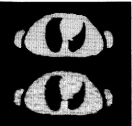
Fig. 1.

backprojection (bottom).

Digital thorax phantom (top), and image reconstructed using filtered

Theorem 1: If the initial iterate po has all components positive, then the sequence p n converges to the global maximum of the log posterior A ( p ) .

Prooj Because the sequence p n is confined to a compact set, it suffices to show that limit set of the sequence reduces to a single point and that this point is the maximum point. Suppose that pm = limk,, pnk is the limit of some subsequence p n h . Let us first show that pm is a station-

ary point of A ( p ) . As noted in c) of Lemma 2, we must demonstrate that all components of pM satisfy either 113" = 0 or ( 3 / d p , ) A ( p " ) = 0. In the nontrivial case p? > 0 , the condition p;"' = epTk cannot hold for infinitely many IC since this would contradict f) of Lemma 3 . Thus pyh+' =

is true for all large IC. It is then clear that the two equations

yield in the limit the desired condition ( d / d p j ) A ( p m ) = 0. Next observe that the limit set of p" is connected because of

assertion e) of Lemma 3 [21]. Since the limit set is contained in the set of stationary points of A ( p ) , and the stationary points are finite in number, connectedness demands that the limit set consist of a single stationary point.

Thus we may assume that limn+, f i n = pm exists. To prove that pLoc is the maximum point, it suffices to verify that each component p y satisfying p? = 0 also satisfies the Kuhn-Tucker condition (d/dpj)A(p,)

5

0 [ l l ] . If

the contrary condition ( a / a p j ) A ( p m )

>

0 holds for such a boundary component, then

holds for all large n. However, this situation entails

[image:6.612.369.500.63.187.2]

(7)

MAP Transmission Algorithms

I 1

1800. 1600. 1400.

m 2 1200-

-

z

-

~ 1 0 0 0 .

m g 800-

n

0" 600- 400 *

+

Gradient Algorithm

X EM Algorithm

-

-I

lnitlalired with FBP Image

ab

0 5 10 15 20

lteratlon

Fig. 2 .

with the FBP image.

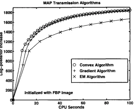
Increase in log-posterior A ( / [ " ) - A ( p o ) versus iteration starting

MAP Transmission Algorlthms

+

X EM Algorithm Initlaiized with FBP Image

0 20 40 60 80 100

CPU Seconds

Fig. 3.

starting with the FBP image.

Increase in log-posterior A(j1") - A ( p 0 ) versus CPU seconds

v.

PERFORMANCE ON SMULATIONS

In this section we describe some representative simulations demonstrating the relative convergence rates of the three algorithms. For these examples, we used the penalized versions (16) and (18) of the algorithms with a simple quadratic smoothing prior of the form

U(,U)

= 7 1

1

WJk(,ULJ - ,Ud2

J kE.k\

where

N3

denotes the usual eight pixel neighborhood of the j t h square pixel. Conventionally one sets the weights W J k

to one for horizontal and vertical neighbors and to l / f i for diagonal neighbors. This choice leads to spatially-variant image resolution, so we used the modified weights described in [4] to make the resolution approximately uniform. We selected the regularization parameter

y

as suggested by Fessler [4] to achieve a resolution of 2.5 pixels or 1.125 cm full-width at half maximum

(FWHM).

For testing the algorithms, we used the synthetic attenuation map shown in Fig. 1, representing a human thorax with

.-

2.8

-

2.6.

+

X EM Algorithm

1

1 I

2.4

initialized with Uniform image

0 5 10 15 20

[image:7.618.310.533.65.252.2]

Iteration

Fig. 4.

with the uniform image.

Increase in log-posterior A(@") - A(@') versus iteration starting

+

Gradient Algorithm 2.6

2.4

Initialized with Uniform Image

0 20 40 60 80 100

CPU Seconds

[image:7.618.50.273.66.247.2]

Increase in log-posterior A ( p n ) - A ( p " ) versus CPU seconds Fig. 5.

starting with the uniform image.

linear attenuation coefficients O.O165/mm, O.O096/mm, and O.O025/mm for bone, soft tissue, and lungs, respectively. The image was decomposed into a 128 by 64 array of 4.5 mm pixels. We simulated a PET transmission scan with 192 radial bins and 256 angles uniformly spaced over 180'. The l ; j factors correspond to 6 mm wide strip integrals on 3 mm center-to-center spacing. (This is an approximation to the ideal line integral that accounts for finite detector width.) The d;

factors were generated using pseudorandom log-normal vari- ates with a standard deviation of 0.3, to zccount for detector efficiency variations, and scaled so that Ci d; exp

(-

( 1 2 , p))

was one million counts. Pseudorandom Poisson transmission projections

Y ,

were generated with means di exp (- ( l ; , ,U)). [image:7.618.309.535.292.479.2] [image:7.618.50.273.294.474.2]

(8)

LANCE AND FESSLER: GLOBALLY CONVERGENT ALGORITHMS 1437

Fig. 6 . Images reconstructed after approximately 15, 30.60, and 110 CPU seconds (left to right) when initialized with the uniform image. Top: iterations 1 , 3, 6, and 1 1 of the EM algorithm. Middle: iterations 4, 12, 24, and 44 of the gradient algorithm. Bottom: iterations 4, 12, 22, and 40 of the convex algorithm.

from a uniform image with attenuation coefficient

0.008/mm.

For the M step of the EM algorithm we employed Newton's method for each parameter [19]. For the gradient algorithm, we enforced monotonicity by repeatedly halving the step size until the objective function increased.

Fig. 2 shows a plot of the increase in the log-posterior A ( p n ) - A ( p o ) function versus iteration n for the algorithms initialized with the FBP image. The computation time per iteration varies among the algorithms, so a more objective comparison is total computation time, which is shown in Fig. 3 as cumulative CPU time as measured on a DEC 3000/800 workstation. The EM algorithm requires

NO

exponentiations per iteration, where NO is the number of nonzero l i j factors

( N O

x 5.6 x lo6 in this case). The convex algorithm and gradient algorithm only require N p exponentiations per iteration, where

N p

is the number of projections

( N ,

=

256 x 192

=

5 x lo4 in this case). Thus, when measured against CPU time, the gradient algorithm and the convex algorithm approach the asymptote of the log-posterior much faster than the EM algorithm (although not 100 times faster since the inner products use much of the time per iteration).

Figs. 4 and 5 are analogous to Figs. 2 and 3 except that here the algorithms are initialized with the uniform image. In this case, the convex algorithm converges faster than the gradient algorithm and the EM algorithm in terms of both CPU time and number of iterations.

It is obvious from these figures that conclusions drawn about convergence rates depend strongly on the starting conditions of the algorithms. In the above cases, the initial

FBP

image has much higher log-posterior than the initial uniform image, and subsequent iterations make smaller changes in the log- posterior. Thus the plots for starting with the FBP image are more related to asymptotic convergence rate, whereas the plots for starting with the uniform image measure initial performance

of

the algorithms

far

from the optimal point.

Maximizing the log-posterior is a surrogate for the real goal of producing better images. Fig.

6

compares the images produced by the three algorithms after 15, 30, 60, and 110 seconds of CPU time. The images from the EM algorithm

are blurry, reflecting slow convergence starting from an initial uniform image. The gradient and convex algorithms produce very similar images and obviously converge much faster than the EM algorithm. As can seen from a comparison of Figs. 1

and 6, the maximum a posteriori images have fewer streak artifacts than the FBP image.

VI. DISCUSSION

Because the EM algorithm for transmission tomography is beginning to see practical application [lS], [19], [23], it is timely to review and compare its performance with competing algorithms. Our limited experience confirms the widespread impression that incorporating a smoothing prior enhances overall image quality. This practical improvement is consistent with the better theoretical behavior of the smoothed algorithms. For instance, sufficient smoothing automatically turns an ill-conditioned maximum likelihood problem into an well-conditioned maximum a posteriori problem.

The smoothed versions of the gradient algorithm

(4)

and the convex algorithm (7) appear to be considerably more efficient than the EM algorithm. This is not surprising in view of the larger number of exponentiations entailed by the EM algorithm. We anticipate that this superiority will continue to hold in other simulation trials. Because we understand its convergence behavior better, we tend to prefer the convex algorithm to the gradient algorithm. [image:8.612.61.541.65.247.2]

(9)

The EM and convex algorithms, and possibly the gradi- ent algorithm as well, could benefit from the quasi-Newton acceleration techniques recently suggested by Lange [ 151.

These techniques attempt to build better approximations to the Hessian d 2 A of the log posterior using the diagonal Hessian

d2Y

of the comparison function

T

as a base. The presence of boundary constraints on the parameters complicates quasi- Newton methods, but perhaps the addition of small barrier terms to the log-likelihood will make acceleration techniques practical without detracting much from the final image.

Although the algorithms discussed here show definite promise, further theoretical improvements are to be expected. At the same time computing costs continue to drop, and processor speeds to increase. These trends imply an accelerating transition away from Fourier methods and toward statistical methods of image reconstruction.

REFERENCES

[ l ] A. P. Dempster, N. M. Laird, and D. B. Rubin, “Maximum likelihood from incomplete data via the EM algorithm,” J . Royal Stat. Soc. Series

[2] A. R. De Plerro, “On the relation between the ISRA and the EM algorithm for positron emission tomography,” IEEE Trans. Med. Imaging,

[3] -, “A modified expectation maximization algorithm for penalized likelihood estimation in emission tomography,” IEEE Trans. Med. Imaging, 1995, to be published.

[4] J. A. Fessler and W. L. Rogers, “Uniform quadratic penalties cause nonuniform image resolution (and sometimes vice versa),” in Proc. I994 IEEE Nucl. Symp. Med. Imaging Con$, 1994.

[5] J. A. Fessler. “Hybrid Poissodpolynomial objective functions for tomographic image reconstruction from transmission scans,” IEEE Trans. Image Processing, this issue, pp. 1439-1450.

[6] S. Geman and D. McClure, “Bayesian image analysis: An application to single photon emission tomography,” in Proc. Stat. Comput. Sec., Amer. Stat. Assoc., Washington, DC, 1985, pp. 12-18.

[7] -, “Statistical methods for tomographic image reconstruction,” IS1 Tokyo session. Bull. Int. Stat. Inst., vol. 52, pp. 5-21, 1987.

[8] P. J. Green, “Bayesian reconstruction for emission tomography data using a modified EM algorithm,” IEEE Trans. Med. Imaging, vol. 9, pp. 84-94, 1990.

[9] -, “On the use of the EM algorithm for penalized likelihood estimation,” J. Royal Srat. Soc. Series E, vol. 52, pp. 4 4 3 4 5 2 , 1990. [lo] G. T. He-, ImaRe Reconstruction from Projections: The Fundamen-

B, vol. 39. pp. 1-38, 1977.

vol. 12, pp. 328-333, 1993.

[13] -, “Convergence of EM image reconstruction algorithms with

Gibbs smoothing,” IEEE Trans. Med. Imaging, vol. 9, pp. 4 3 9 4 4 6 , corrections IEEE Trans. Med. Imuging, vol. 10, p. 228, 1990.

[ 141 __ , “A gradient algorithm locally equivalent to lhe EM algorithm,”

J. Royal Stat. Soc. Series E, vol. 57, pp. 4 2 5 4 3 7 , 1995.

[ 151 __, “A quasi-Newton acceleration of the EM algorithm,” Statistica Sinica, vol. 5, pp. 1-18, 1995.

[ 161 K. Lange, M. Bahn, and R. Little, “A theoretical study of some maximum likelihood algorithms for emission and transmission tomography,” lEEE Trans. Med. Imaging, vol. 6, pp. 106-114, 1987.

[ 171 K. Lange and R. Carson, “EM reconstruction algorithms for emission and transmission tomography,” J. Comput. Assist Tomog., vol. 8, pp. 306-316, 1984.

[l8] S. H. Manglos, F. D. Thomas, G . M. Gagne, and B. J. Hellwig, “Phantom study of breast tissue attenuation in myocardial imaging,” J . Nucl. Med.,

[ 191 J. M. Ollinger, “Maximum likelihood reconstruction of transmission images in emission computed tomography via the EM algorithm,” IEEE Trans. Med. Imaging. vol. 13, pp. 89-101, 1994.

[20] J. M. Ortega, Numerical Analysis: A Second Course. Philadelphia, PA: SIAM, 1990, pp. 144-145.

[21] J. M. Oitega and W. C. Rheinboldt, Iterative Solution of Nonlinear Equations in Several Variables.

[22] A. M. Ostrowski, Solutions of Equations in Euclidean and Banach Spaces.

[23] L. A. Shepp and Y. Vardi, “Maximum likelihood reconstruction for emission tomography,” IEEE Trans. Med. Imuging, vol. 1, pp. 1 13-1 21, 1982.

[24] C. H. Tung, G. T. Gullherg, G. L. Zing, P. E. Christian, F. L. Datz, and H. T. Morgan, “Nonuniform attenuation correction using simultaneous transmission and emission converging tomography,” IEEE Trans. Nucl. Sci., vol. 39, pp. 11341143, 1992.

[25] Y. Vardi, L. A. Shepp, and L. Kaufman, “A statistical model for positron emission tomography,” J. Amer. Slat. Assoc., vol. 80, pp. 8-37, 1985. vol. 34, pp. 992-996, 1993.

New York: Academic, 1970.

New York: Academic, 1973, p. 173.

Kenneth Lange is Professor of Biostatistics at the University of Michigan. After graduating from Michigan State University in 1967, he pursued the Ph.D. degree in mathematics at the Massachusetts Institute of Technology. During the 1971-1972 academic year, he served as an assistant professor at the University of New Hampshire. From 1972-1994, he was affiliated with the Department of Biomathe- matics at the University of California, Los Angeles, where he eventually became professor and department chair. His research interests include human

~~

tals of Computerized Tomography.

[ l 11 M. R. Hestenes, Optimization Theory: The Finite Dimensional Case. Huntington, NY: Krieger, 1981, pp. 186 and 2 3 e 2 3 4 .

[12] K. Lange, “An overview of Bayesian methods in image reconstruction,” in Digital Image Synthesis and Inverse Optics. A. F. Gmitro, P. S. Idell, and I. S. La Haie, Eds., Society of Photo-Optical Engineering, Bellingham, WA, SPIE, vol. 1351, 1990, pp. 27C-287.

New York: Springer, 1980. genetics, population biology, biomedical imaging, computational statistics, and applied stochastic processes.

Jeffrey A. Fessler, for a photograph and biography, see this issue, p. 1450.