Improving surface tidal accuracy through two way nesting in a global ocean model

Contents lists available atScienceDirect

Ocean Modelling

journal homepage:www.elsevier.com/locate/ocemod

Improving surface tidal accuracy through two-way nesting in a global ocean

model

Chan-Hoo Jeon

_{, Maarten C. Buijsman}

_{, Alan J. Wallcraft}

_{, Jay F. Shriver}

_{, Brian K. Arbic}

_,

James G. Richman

_{, Patrick J. Hogan}

a_{Division of Marine Science, The University of Southern Mississippi, Stennis Space Center, MS, USA} b_{Center for Ocean-Atmospheric Prediction Studies, Florida State University, Tallahassee, FL, USA} c_{Oceanography Division, Naval Research Laboratory, Code 7323, Stennis Space Center, MS, USA} d_{Department of Earth and Environmental Sciences, University of Michigan, Ann Arbor, MI, USA}

A R T I C L E I N F O

Keywords:

Two-way nesting HYCOM Barotropic tides OASIS3-MCT FES2014 TPXO9-atlas

A B S T R A C T

In global ocean simulations, forward (non-data-assimilative) tide models generally feature large sea-surface-height errors near Hudson Strait in the North Atlantic Ocean with respect to altimetry-constrained tidal solu-tions. These errors may be associated with tidal resonances that are not well resolved by the complex coastal-shelf bathymetry in low-resolution simulations. An online two-way nesting framework has been implemented to improve global surface tides in the HYbrid Coordinate Ocean Model (HYCOM). In this framework, a high-resolution child domain, covering Hudson Strait, is coupled with a relatively low-high-resolution parent domain for computational efficiency. Data such as barotropic pressure and velocity are exchanged between the child and parent domains with the external coupler OASIS3-MCT. The developed nesting framework is validated with semi-idealized basin-scale model simulations. The M2sea-surface heights show very good accuracy in the

one-way and two-one-way nesting simulations in Hudson Strait, where large tidal elevations are observed. In addition, the mass and tidal energy flux are not adversely impacted at the nesting boundaries in the semi-idealized si-mulations. In a next step, the nesting framework is applied to a realistic global tide simulation. In this simulation, the resolution of the child domain (1/75°) is three times as fine as that of the parent domain (1/25°). The M2

sea-surface-height root-mean-square errors with tide gauge data and the altimetry-constrained global FES2014 and TPXO9-atlas tidal solutions are evaluated for the nesting and no-nesting solutions. The better resolved coastal bathymetry and the finer grid in the child domain improve the local tides in Hudson Strait and Bay, and the back-effect of the coastal tides induces an improvement of the barotropic tides in the open ocean of the Atlantic.

1. Introduction

Global surface tides have been studied in barotropic (two-dimen-sional) and baroclinic (three-dimen(two-dimen-sional) forward and data-assim-ilative simulations (Arbic et al., 2004; Arbic et al., 2009; Buijsman et al., 2015; Egbert and Ray, 2001; Egbert et al., 2004; Green and Nycander, 2013;Ngodock et al., 2016;Shriver et al., 2012;Stammer et al., 2014). Despite recent progress in reducing tidal sea-surface-height root-mean-square errors (RMSE) in the global HYbrid Co-ordinate Ocean Model (HYCOM), the model used in this paper, the errors in the North Atlantic near Hudson Strait, and near coastal-shelf areas in general, are still relatively large (Buijsman et al., 2015; Ngodock et al., 2016;Shriver et al., 2012). Coastal-shelf bathymetry is imperfectly known and represented in models, and may be a likely

cause of tidal model errors (Egbert et al., 2004). Moreover, the large errors in the North Atlantic may be attributed to the inability of the model to correctly simulate the known semidiurnal tidal resonances in the North Atlantic (Wünsch, 1972).

Both analytical models of coastal tides (e.g. the classic quarter-wa-velength resonance model, see for instanceDefant, 1961) and more realistic numerical models of coastal tides have long treated the open ocean as representing an unchanging boundary condition acting on a coastal region that may or may not achieve resonance depending on its geometry. However, in analytical and numerical studies,Arbic et al. (2009),Arbic et al. (2007), andArbic and Garrett (2010)have shown that there is a substantial “back-effect” of coastal tides upon the open-ocean tides. They showed that if both the shelf sea and open-ocean basin are near resonance, small geometry changes to the shelf sea can have a

https://doi.org/10.1016/j.ocemod.2019.03.007

Received 7 May 2018; Received in revised form 19 March 2019; Accepted 23 March 2019

⁎_{Corresponding author at: Naval Research Laboratory, Code 7323, Bldg. 1009, Stennis Space Center, MS 39529, USA.} E-mail address:[email protected](C.-H. Jeon).

Available online 04 April 2019

1463-5003/ © 2019 Elsevier Ltd. All rights reserved.

large impact on the open-ocean tides. This suggests that if we better resolve the coastal geometry by increasing the model resolution, we may not only improve the coastal tides, but also the open-ocean tides through the back-effect, in particular if the shelf and ocean basins are near resonance, as is the case in the North Atlantic near Hudson Strait. In general, higher resolution yields more accurate tides in forward models (Egbert et al., 2004). However, high-resolution model simula-tions are computationally expensive and require large data storage. To achieve higher resolution in regions of interest without dramatically increasing the cost of a basin- or global-scale model, one can use two-way nesting, as introduced inSpall and Holland (1991). The basic idea of two-way nesting is to apply a high-resolution (fine) grid only to a small area of interest, i.e., the ‘child’ domain, and a low-resolution (coarse) grid to the entire ‘parent’ domain. In two-way nesting, in-formation is allowed to propagate from the coarse grid to the fine grid and vice versa. In this way, the improved solution on the child grid may also improve the solution on the parent grid. In this paper, we imple-ment a two-way nesting framework for barotropic HYCOM simulations to better simulate the local surface tides, e.g. on Hudson shelf, as well as the remote tides in the open ocean.

In the two-way nesting framework, the data exchange between the child and parent domains occurs in two opposing directions. In the first ‘coarse-to-fine’ direction, the information of the parent domain is transferred to the child domain via the lateral boundaries of the child domain. Data exchange in this direction is also referred to as ‘one-way nesting’. In one-way nesting, the parent domain is not updated with the child grid solution. One-way nesting has been extensively used for basin-scale modeling (Chassignet et al., 2007; Hogan and Hurlburt, 2006;Mason et al., 2010;Penven et al., 2006). In the second ‘fine-to-coarse’ direction, the coupling variables in the high-resolution child domain are transferred to the relatively low-resolution parent grid. The two-way nesting approach has been widely applied in atmospheric modeling (Bowden et al., 2012;Lorenz and Jacob, 2005), and in cou-pling of multiple climate models (Lam et al., 2009;Ličer et al., 2016; Wahle et al., 2017) as well as ocean modeling (Barth et al., 2005; Debreu et al., 2012;Ginis et al., 1998). To make the updated variables continuous across the nesting boundaries of the parent and child do-mains in the second direction, smoothing filters were sometimes ap-plied to physical variables, and/or the bottom topography of the child domain was relaxed with that of the parent domain (Debreu et al., 2012;Fox and Maskell, 1995;Ginis et al., 1998;Mason et al., 2010). The artifacts at the nesting boundary are amplified when the grid-re-solution ratio of the child and parent domains increases (Spall and Holland, 1991). In this study, barotropic pressure, velocity, and bottom topography are linearly relaxed near the boundary of the child domain to allow for a smooth transition of these data between the child and parent domains, which the grid-resolution ratio is three.

The two-way nesting approaches can be classified into two cate-gories: (i) internal, and (ii) external coupling. In internal coupling, a nesting framework is included in the source code of ocean models (Barth et al., 2005;Debreu and Blayo, 2008;Haley Jr. and Lermusiaux, 2010; Herrnstein et al., 2005; Santilli and Scotti, 2015;Tang et al., 2014). This approach requires more complicated nesting algorithms than a single resolution (no-nesting) case. In external coupling, a se-parate coupler facilitates the communication between numerical models. The main advantage of using such a coupler is that the mod-ification of the source code of these models is minimal. It is only ne-cessary that the Application Programming Interface (API) of the coupler be built into the existing source codes. In addition, external couplers provide a wide variety of interpolation schemes and efficient search algorithms that can be used to calculate interpolation (remapping) coefficients. The data that are transferred between coupled models need to be interpolated for use in the destination domain because the grid cells in the destination domain may not be located at the same co-ordinates as the grid cells in the source domain. Several external cou-plers have been developed and applied (Valcke et al., 2012). The Earth

System Modeling Framework (ESMF) can be used to couple multiple domains with different resolutions (Qi et al., 2018). In recent research, the AGRIF and OASIS3-MCT coupling toolkits have been widely ap-plied. The AGRIF (Adaptive Grid Refinement In Fortran) coupler has been used to couple ocean circulation models (Debreu et al., 2012; Penven et al., 2006; Urrego-Blanco et al., 2016). The OASIS3-MCT coupler (Valcke et al., 2015) has been used to couple climate models (Juricke et al., 2014;Ličer et al., 2016;Wahle et al., 2017;Will et al., 2017). OASIS3-MCT is an integrated version of OASIS3 (Ocean Atmo-sphere Sea Ice and Soil) by CERFACS in France and MCT (Model Cou-pling Toolkit) by the Argonne National laboratory in USA. We utilize OASIS3-MCT as a coupler for the HYCOM to HYCOM two-way nesting because its partition option, grid and mask, and parallel computing by Message Passing Interface (MPI) are more compatible with HYCOM as compared to AGRIF. Scientists at the Service Hydrographique et Océanographique de la Marine (SHOM; Brest, France) applied AGRIF to facilitate the HYCOM to HYCOM coupling, but found it hard to main-tain as the HYCOM code was updated (personal communication with Remy Baraille, 2015).

HYCOM provides reliable results as a multi-layer global ocean cir-culation model and contributes to the United States Navy's operation (Arbic et al., 2010; Chassignet et al., 2007; Metzger et al., 2010; Ngodock et al., 2016;Shriver et al., 2012). The forward barotropic tide simulations (single layer), used in this paper, employ astronomical tidal forcing, a spatially-varying self-attraction and loading (SAL) term, a linear topographic wave drag (Buijsman et al., 2015), and an atmo-spheric mean sea level pressure forcing, which modulates the S2tide

and is obtained from the atmospheric NAVGEM (NAVy Global En-vironmental Model;Hogan et al., 2014). HYCOM is also capable of improving basin-scale modeling with offline one-way nesting (Chassignet et al., 2007; Hogan and Hurlburt, 2006). However, the offline one-way nesting in HYCOM has some drawbacks. First, it re-quires additional data storage for nesting data, whose size increases proportionally to the resolution of the computational domain. Second, global-scale modeling on the parent grid must be performed in advance of regional/basin-scale modeling on the child grid to provide boundary conditions for the child domain. Third, offline one-way nesting is useful only for improving the solution in the child domain, while the parent domain does not receive any feedback from the child domain. Anonline two-waynesting framework is able to resolve these issues and improve the accuracy in HYCOM for both regional/basin- and global-scale modeling. The most complicated issue in applying OASIS3-MCT to HYCOM is how to deal with barotropic time stepping in conjunction with the baroclinic time steps that are based on the second-order leapfrog scheme. This study synchronizes nesting variables at the bar-otropic time steps of the parent domain without any other treatments (Santilli and Scotti, 2015;Urrego-Blanco et al., 2016), and stores them so that they can be used at the next baroclinic time level.

Stammer et al. (2014).

This paper is organized as follows. The online two-way nesting framework in HYCOM is described inSection 2. The developed nesting framework is validated with semi-idealized basin-scale simulations in Section 3. The framework is then applied to a realistic global-scale si-mulation and validated against tide gauge data, FES2014, and TPXO9-atlas inSection 4. Finally, we end with a discussion and conclusions in Section 5.

2. Methodology: OASIS3-MCT in HYCOM

2.1. Data exchange in HYCOM

In solving the layer-integrated nonlinear momentum equations, HYCOM uses a split-explicit time-stepping scheme that separates the fast barotropic mode (single layer) from the slow baroclinic modes (multiple layers) for numerical efficiency (Bleck and Smith, 1990). In barotropic HYCOM simulations, as in this paper, this split-explicit time-stepping scheme is still used. In this case, HYCOM performs the cal-culations over two layers: a surface layer with a varying thickness and a bottom layer with a zero thickness. Hence, we need to prescribe a barotropic time step (ΔtT) and a baroclinic time step (ΔtC). Since

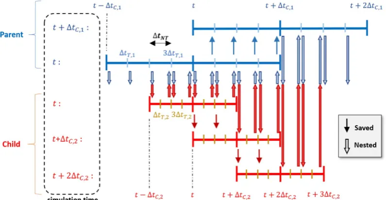
bar-otropic waves have larger phase speeds than baroclinic waves, the barotropic time step is much smaller than the baroclinic time step. The split-explicit scheme is computationally efficient because the two-di-mensional calculations occur on the fast time step and the more ela-borate three-dimensional calculations occur on the longer time step. An example of the barotropic and baroclinic time stepping is shown in Fig. 1for both the parent and child domains. Time is integrated with the second-order leapfrog scheme for the baroclinic mode, and with a combination of the first-order forward and backward Euler schemes for the barotropic mode (Bleck and Smith, 1990). The leapfrog scheme is a two-step method that uses two baroclinic time steps of (t− ΔtC) andtto

evaluate the values at (t+ ΔtC) wheretdenotes a certain simulation

time. This means that one of two baroclinic time steps is overlapped every baroclinic calculation (Fig. 1). In this study, the data of the second baroclinic time step of the previous simulation time (t) are stored in memory, and the saved data are used in the first baroclinic time step of the next simulation time (t+ ΔtC). This method, in which

the stored data for one baroclinc time step is used, is more efficient than exchanging data from (t− ΔtC) and (t+ ΔtC) every simulation time.

In general, the baroclinic and the barotropic time steps of a parent

domain (ΔtC, 1and ΔtT, 1) are different from those of a child domain

(ΔtC, 2and ΔtT, 2) because the stable time step for a fine grid is smaller

than that for a coarse grid based on the CFL (Courant-Friedrichs-Lewy) condition (Figs. 1 and 2). As shown inFig. 2, the barotropic long-itudinal and latlong-itudinal velocities, and the barotropic pressure are transferred in the firstcoarse-to-finedirection before solving the con-tinuity equation, and in the secondfine-to-coarsedirection after com-puting the momentum equations. In HYCOM, two barotropic time steps are calculated in a pair to improve the numerical stability in calculating the momentum equations with the Coriolis force (Bleck and Smith, 1990). The child domain can receive data every barotropic time step from the parent domain (ΔtT, 2), but no data are sent from the parent

domain in the case that the barotropic time steps of the parent and the child domains do not coincide. InFigs. 1 and 2, for example, the bar-otropic (ΔtT, 1) and the baroclinic (ΔtC, 1) time steps of the parent

do-main are twice as large as those (ΔtC, 2and ΔtT, 2) of the child domain.

In this case, data are exchanged in both directions every other baro-tropic time step of the child domain as the nesting time step (ΔtNT). This

means that the nesting variables are synchronized at the end of the barotropic time step of the parent domain (ΔtNT= ΔtT, 1= 2ΔtT, 2).

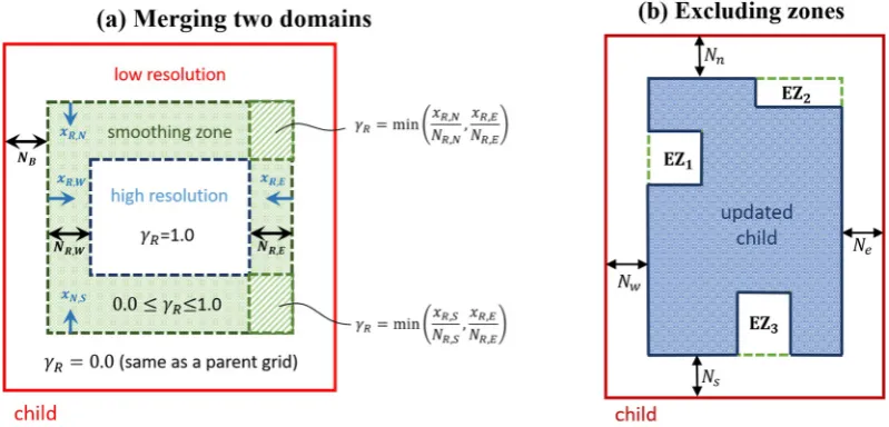
The data from the parent domain are used as a lateral boundary condition for the child domain in the first direction. However, the difference in grid resolution between the two domains may create discontinuities in the topography along the domain boundaries. To prevent this, it is necessary to match the topography of the parent domain with that of the child domain along the boundary of the child domain. As shown inFig. 3a, the bottom topography of the child do-main is divided into three zones. The outermost zone (width:NB) uses

the low-resolution bottom topography that is the same as that of the parent domain while the innermost zone uses the high-resolution bottom topography. The smoothing zone in the middle merges the low-and high-resolution topographies as

= _R· _child+(1.0 _R)· _{parent (1)}

whereϕis the bottom topography, andγRis the relaxation factor that is

linearly evaluated by

= x =

N l N S E W min , { , , , or }

R R l

R l ,

, (2)

whereNR,lis the number of cells in the width of the smoothing zone,

andxR,lis the cell number as counted from the outer north, south, east,

Fig. 1.The split-explicit time stepping scheme for both the parent and child domains. The barotropic and baroclinic time steps are ΔtTand ΔtC, respectively. Data are

and west boundaries. Other physical variables such as barotropic pressure and velocity are also relaxed in the same manner.

In addition, to avoid instabilities at the boundary of the child do-main in the second direction, a specified number of boundary cells in the child domain (Ne,Nw,Nn, andNs) are not updated along the eastern,

western, northern, and southern boundaries as shown in Fig. 3b. Moreover, cutting off a parent domain sometimes results in isolated ocean cells near the boundary of a child domain. As HYCOM requires that all ocean cells should be connected as one sea, these isolated ocean cells are modified into land cells. This means that OASIS3-MCT does not have any remapping coefficients and data are not transferred to these ocean cells. Therefore, the area updated in the second direction should exclude these isolated ocean areas (EZ). The data in the blue zone in Fig. 3b are only exchanged between the parent and child domains.

2.2. Remapping files of OASIS3-MCT

In transferring data with OASIS3-MCT, remapping files for each direction and variable are required. The remapping files for

OASIS3-MCT contain information on the coupling direction, the grids involved in the exchange direction, the interpolation coefficients, and the ad-dress information of a target point on the destination grid and its four neighboring points on the source grid. HYCOM is based on the stag-gered Arakawa C-grid (Bleck and Smith, 1990). The scalar variables such as pressure, temperature, and salinity are stored at the center of a computational cell (p-grid), while the longitudinal and latitudinal ve-locities are stored at the center of the western side (u-grid) and the southern side (v-grid) of a computational cell, respectively. Table 1 shows the nesting variables and their base grids for each direction whereP,U, andVdenotep-,u-, andv-grids, respectively. In the first

direction, the lateral boundary condition ofBrowning and Kreiss (1982) is applied on the p-grid for the barotropic pressure and velocity. Therefore, the barotropic pressure on the p-grid and the barotropic velocity fields on the u- andv-grids of the parent domain are inter-polated onto thep-grid along the boundary of the child domain. In the second direction, the barotropic variables of pressure and velocity in the child domain are interpolated onto the same types of grids in the parent domain.

Fig. 2.Data exchange between parent and child domains in two sequential barotropic time steps in the parent domain.

Fig. 3.Boundary zones in the child domain. (a) Inside the child domain, the low resolution parent bathymetry is used near the boundary over a width ofNBcells. The

child and parent bathymetries are merged in the smoothing zones (NR,l). (b) Data in the excluding zones (NandEZ) are not used for updating the parent domain in the

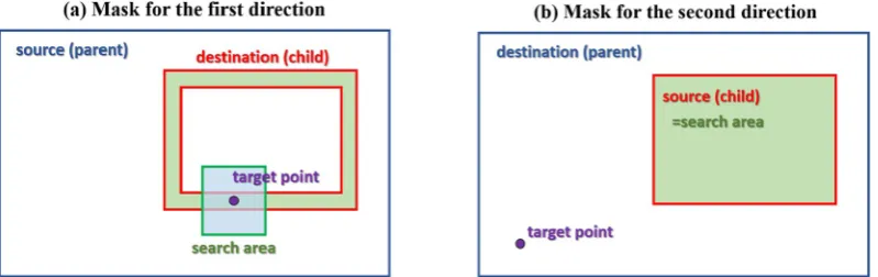
In computing the remapping coefficients, OASIS3-MCT searches the entire parent grid, which may take a long time. Will et al. (2017) suggested that the masks of the ocean cells located outside the child domain be modified into land in the second direction. If the target point is a land cell, this calculation is skipped in OASIS3-MCT, reducing the computing time for the remapping coefficients. In this study, the ap-proach byWill et al. (2017)is applied to both the first and the second directions. In the first direction, we not only modify most of the child domain into land cells except for the boundary cells, but also set limits to the search algorithm. Since the data coming from the parent domain are used as the boundary condition for the child domain, only boundary ocean cells in the child domain require data in the first direction. As shown inFig. 4a, a specific number of boundary cells (green, 5 cells from the boundary) are active while the other inner ocean cells in the child domain (white) are changed to land cells. In order to calculate remapping coefficients for a target point in the destination (child) do-main, OASIS3-MCT searches for four surrounding points of each target point in the source (parent) domain. Instead of including all the parent grid points in the search, we limit the search to a small area (light blue box) around the ocean cell in the parent domain corresponding to the target point in the child domain (Fig. 4a). In this study, the search box has 20 grid points in the parent domain in both longitudinal and lati-tudinal directions. This box follows the target point in the child domain as it moves eastward or northward. The efficiency of this approach is shown inTable 2. Three regions (ARC, HUD, and GLB), which are used inSections 3 and 4, are involved in the calculation. The modified ap-proach significantly reduces the computing time by at least an order of magnitude as compared to the original method.

In the second direction, only ocean cells that are located inside the child region are updated in the parent domain. As illustrated inFig. 4b, the remapping coefficients for the target points that are located outside the child region are not necessary in two-way nesting. By modifying the masks of the ocean cells outside the child area into land cells, the computing time of creating the remapping files for the second direction

significantly decreases by several orders of magnitude as shown in Table 3.

3. Validation of the nesting framework

The developed nesting framework is validated with six semi-idea-lized model simulations. Experiments 1–2 concern one-way nesting and Experiments 3–6 concern two-way nesting. The parent and child grid resolutions are the same in Experiments 1–4, while they differ in Experiments 5–6. Experiment pairs 1–2, 3–4, and 5–6 concern the sensitivity to equal and different time steps on the parent and child grids. The grid resolutions and time steps of the parent and child do-mains in Experiment 6 are the same as those of the global experiment, discussed in the next section. The specifications of Experiments 1–6 are presented inTables 4 and 5.

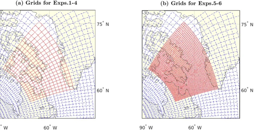
The HUD child domain, covering Hudson Strait, and the ARC parent domain are shown inFig. 5. The parent domain covers the Arctic and the North Atlantic Oceans rather than the entire global ocean for computational efficiency. For Experiments 1–4, the grid resolution of both the child and parent domains is 1/25°_{. To ensure the child grid is}

identical to the parent grid in Experiments 1–4, the child domain is extracted from the parent domain (Fig. 6a). For Experiments 5 and 6, the child grid has a resolution of 1/75°_{, which is three times as fine as}

the parent grid (Fig. 6b). In case that the refinement ratio between parent and child domains is odd, the interpolation error is reduced because the grid points on thep-,u-, andv-grids of the parent domain Table 1

Base grids of data exchange on the HYCOM C-grid for OASIS3-MCT remapping files (P:p-grid,U:u-grid, andV:v-grid).

No. Variable name Parent Direction Child

First direction: parent (coarse) → child (fine)

1 Barotropic pressure P → P

2 Barotropicu-velocity U → P

3 Barotropicv-velocity V → P

Second direction: child (fine) → parent (coarse)

1 Barotropic pressure P ← P

2 Barotropicu-velocity U ← U

3 Barotropicv-velocity V ← V

Fig. 4.Masks for computing remapping coefficients. (a) In the first direction, the calculation in the child domain (destination) is limited to a small green area along its boundary, and the search for four neighboring points of a target point in the parent domain (source) is limited to the blue box. (b) In the second direction, the computation is limited to parent grid cells located inside the child region (green), and all parent grid cells outside the child domain are masked as land (white). (For interpretation of the references to color in this figure legend, the reader is referred to the web version of this article.)

Table 2

Wall-clock time for the one-time calculation of remapping files for the first direction for the ARC, HUD, and GLB configurations.

Number of cells Computing time

Parent Child Original Modified

3200 × 5040 (ARC) 658 × 1015 (HUDa) 4.07 h 12.12 min 3200 × 5040 (ARC) 1975 × 3046 (HUDb) 2.06 d 1.62 h 9000 × 7055 (GLB) 1975 × 3046 (HUDb) 10.02 d 1.82 h

Table 3

Wall-clock time for computing remapping files for the second direction for the ARC, HUD, and GLB configurations.

Number of cells Computing time

Parent Child Original Modified

are located at the same grid points of the child domain. In Experiments 1–4, the child domain has 658 cells in the longitudinal direction and 1015 cells in the latitudinal direction, while in Experiments 5 and 6 the child domain has 1975 cells in the longitudinal direction and 3046 cells in the latitudinal direction (Table 4). The number of computational cells in the parent domain is 3200 × 5040 for all the experiments. The child domain runs on 128 MPI processes, and the parent domain is partitioned in 320 MPI processes.

The barotropic and baroclinic time steps of the parent domain are

ΔtT= 3.0 s and ΔtC= 60.0 s in all experiments, except in Experiment 5,

which features ΔtT= 1.0 s and ΔtC= 20.0 s (Table 5). The nesting time

step (ΔtNT) is the same as the barotropic time step of the parent domain

in all experiments. In Experiments 1, 3, and 5, the barotropic and baroclinic time steps of the child domain are the same as those of the parent domain. In Experiments 2, 4, and 6, the barotropic and bar-oclinic time steps of the child domain are a third of those of the parent domain, i.e., ΔtT= 1.0 s and ΔtC= 20.0 s.

In Experiments 1–6, the number of cells excluded in the second direction (Nn,s,e,w) is 5 to 10 cells to prevent errors at the boundary of

the child domain from propagating into the parent domain. In all two-way nesting experiments, the width of the zone with the low-resolution parent bathymetry isNB= 10 cells and the width of the smoothing

(relaxation) zone isNR= 10 cells.

The simulations start from rest in all the experiments. The M2

bar-otropic tide is forced at the southern boundary of the parent domain. The only forcing of the child domain comes from the parent domain through the lateral boundary. No atmospheric forcing is applied in all the simulations. The boundary forcing and the identical grids in Experiments 1–4 provide two advantages as a validation case. First, the result of the parent domain without any nesting can be used as the ‘true’ reference solution. In the experiments with identical grid-resolution and two-way nesting (Experiments 3 and 4), the two-way nesting result computed in the parent domain should be the same as the reference solution because the parent domain does not obtain any improvement from the same-resolution child domain. This means that the difference between the nesting and the no-nesting solutions represents the nu-merical error caused by the nesting communication. The resolution of the child domain is not the same as that of the parent domain in Experiments 5 and 6. Since the higher-resolution child domain gen-erally returns more accurate results to the parent domain, the no-nesting solution is not valid as the true solution. Hence, we focus on discontinuities and errors near the updated boundaries in the parent domain in Experiments 5 and 6. Second, the performance of the lateral boundary condition of the child domain can be validated with one-way nesting (Experiments 1 and 2). The child domain receives forcing only through the lateral boundary in the firstcoarse-to-finedirection but does not send back any data to the parent domain in the secondfine-to-coarse direction. The difference between the numerical results in the child domain and the no-nesting solution informs us about the accuracy of Table 4

Specifications of the child and parent domains for the semi-idealized model experiments.

Child (HUD) Parent (ARC)

Experiment number 1–4 5–6 1–6

Grid resolution (°) 1/25 1/75 1/25

Number of cells 658 × 1015 1975 × 3046 3200 × 5040

Number of MPI Processes 128 128 320

OASIS3-MCT interpolation Bi-linear Bi-linear Bi-linear

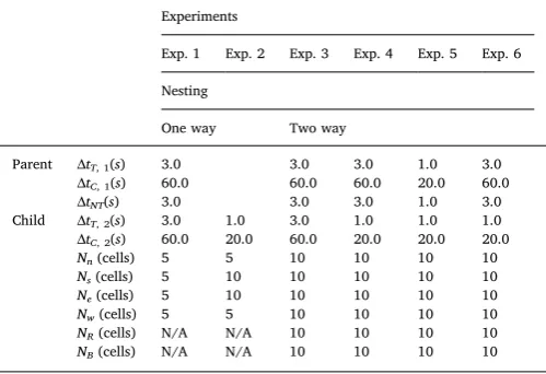
Table 5

Time steps and excluding zones for the six semi-idealized experiments.

Experiments

Exp. 1 Exp. 2 Exp. 3 Exp. 4 Exp. 5 Exp. 6

Nesting

One way Two way

Parent ΔtT, 1(s) 3.0 3.0 3.0 1.0 3.0

ΔtC, 1(s) 60.0 60.0 60.0 20.0 60.0

ΔtNT(s) 3.0 3.0 3.0 1.0 3.0

Child ΔtT, 2(s) 3.0 1.0 3.0 1.0 1.0 1.0

ΔtC, 2(s) 60.0 20.0 60.0 20.0 20.0 20.0

Nn(cells) 5 5 10 10 10 10

Ns(cells) 5 10 10 10 10 10

Ne(cells) 5 10 10 10 10 10

Nw(cells) 5 5 10 10 10 10

NR(cells) N/A N/A 10 10 10 10

NB(cells) N/A N/A 10 10 10 10

the lateral boundary conditions in HYCOM.

In Experiments 1–4, the accuracy over the parent domain is eval-uated with the sea-surface-height root-mean-square error between the nesting result and the no-nesting reference solution at each computa-tional cell

= =

N

RMSEi j n ( )

N

i jn i jn , 1 , ,

2

(3) whereηis the sea-surface height (SSH) of the nesting solution, is the

SSH of the reference solution,n is the temporal order of the hourly saved data,Nis the total number of output data, andiandjare the computational cell indexes along the longitudinal and latitudinal di-rections, respectively. To exclude a spin-up error, only data between days 3 and 5 are used in the calculation. Eq.(3)represents the time-averaged absolute error with the reference solution. The relative error can be estimated with the normalized root-mean-square error

=

NRMSi j RMSEi j i j

, ,

, (4)

where

= =

N ( )

i j n

N i jn

, 1 ,

2

(5) is the standard deviation of the sea-surface heights.

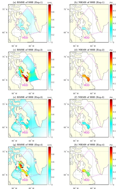
The sea-surface-height root-mean-square errors (RMSE) and the normalized errors (NRMS) with the reference solution for Experiments 1–4 are shown in Fig. 7. In these experiments, the resolutions of the parent and child grids are identical. The standard deviation of the sea-surface heights in the parent domain for the no-nesting reference so-lution is illustrated inFig. 8. The NRMS values inFig. 7are plotted only in the Hudson Strait region where relatively large sea-surface heights are observed. InFig. 7a and b, the RMSE values for Experiment 1 are mostly < 2.0 mm over the child domain (HUD), and the NRMS values are < 0.1% in the Hudson Strait region. This result indicates that the lateral boundary condition of the child domain works accurately. Fig. 7c and d shows RMSE and NRMS for Experiment 2, in which the parent and child-grid time steps differ. Even though these RMSE and NRMS values are larger than those of Experiment 1, the accuracy is still

quite good with errors < 0.5% in the Hudson Strait region. The errors of Experiment 2 are larger than those of Experiment 1 because the data are exchanged between the parent and child domains only at the nesting time steps (ΔtNT= 3.0 s), and errors are accumulated at the

other two barotropic time steps (ΔtT, 2) in the child domain. The

nu-merical errors of the two-way nesting experiments are expected to be larger than those of the one-way nesting experiments because the two-way nesting performs one more communication for the second direc-tion, and there should be no accuracy improvement in the child domain with identical grid resolution. The RMSE and NRMS values for Ex-periment 3 inFig. 7e and f are < 5.0 mm and 0.2% in the Hudson Strait region, respectively. As expected, these errors are slightly larger than those of the one-way nesting Experiment 1. However, for Experiment 4, with different parent- and child-grid time steps (Fig. 7g and h), the errors are reduced compared to Experiment 2 (< 7.0 mm and 0.35%) due to unknown causes. We do not observe significant error accumu-lations along the boundaries of the child domain in Experiments 3 and 4 (Fig. 7e and g).

To study how the two-way nesting affects the propagation of phy-sical variables, in particular near the nesting boundaries and smoothing zones, we calculate for Experiments 3–6 the mass flow rate

= + u

m ( H) , ₍₆₎

the residual of the continuity

= + + u

R

t ·( H) , (7)

and the barotropic energy fluxes (Egbert and Ray, 2001)

=

F ( gH )u (8)

whereρis the water density (=1036.31 kg/m3_{),uis the barotropic}

velocity vector, η is the sea-surface height, H is the water depth,

F= (Fx,Fy) is the energy flux vector,FxandFyare the longitudinal and

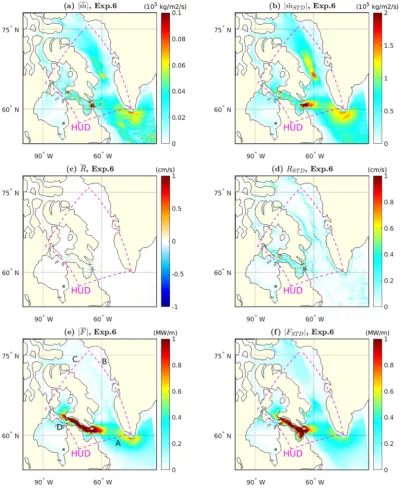
latitudinal components, andgis the gravitational coefficient (=9.81 m/ s2_{). The magnitude of the time-mean and the standard deviation of the}

mass flow rate vectors and energy flux vectors, and the time-mean and the standard deviation of the continuity residual for Experiment 6 are presented inFig. 9. The results for Experiments 3–6 are nearly identical, and similar figures for Experiments 3–5 are not shown. The difference Fig. 6.Grid resolution of the parent domain (blue dashed lines) and the child domain (red solid lines) for (a) Experiments 1–4, in which the parent and child grids have the same resolution, and (b) Experiments 5 and 6, in which the parent and child grids have a resolution of 1/25°_{and 1/75}°_{, respectively. (For interpretation of}

in time steps between Experiments 3 and 4 and Experiments 5 and 6 causes relative differences in the mass flow rate, continuity, and energy fluxes in the parent solution updated with the child solution that are generally smaller than 1%. The mean and the standard deviation of the residual inFig. 9c and d have larger values near topographic gradients, as opposed to the nesting boundaries. In all two-way nesting experi-ments, mass is conserved across the south, west, north, and east boundaries. There are no obvious indications that the nesting bound-aries trap, reflect, and diffract the tidal waves. This is further illustrated in Fig. 10, which shows the time-averaged tidal energy flux in the parent domain integrated along the cells parallel to the boundaries for Experiments 3–6. Compared to the reference (no-nesting) solution, the tidal energy flux is conserved in all experiments. Since the comparisons for the mass flow rate and the continuity residual show the same smooth transition as that of the tidal energy flux, they are not shown here.

In this section, we have tested the performance of the developed two-way nesting framework with six semi-idealized experiments for various time steps and grid resolutions. We conclude that the two-way nesting framework works with a high accuracy, and the tidal energy and mass are conserved quite well.

4. Global barotropic tides

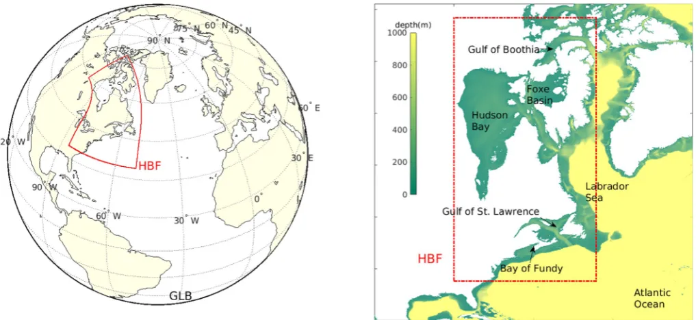
To improve the tidal accuracy in the global HYCOM simulations, we apply the two-way nesting framework to a high-resolution child domain (1/75°) and a relatively low-resolution global parent domain (1/25°). The child domain, referred to as HBF, and its surroundings are shown in Fig. 11. Since the southeast entrance of Fury and Hecla Strait is blocked as land in the relatively low-resolution (1/25°) domain, and Hudson Bay plays an important role in the resonance of the M2barotropic tide

in Hudson Strait (Arbic et al., 2007), the child domain in this realistic experiment is moved westward and extended to Hudson Bay, Rose Welcome Sound, and Fury and Hecla Strait. Moreover, the child domain is expanded southward to include the Bay of Fundy and Gulf of St. Lawrence regions that feature large tides and sea-surface-height root-mean-square errors. The southward expansion ensures that additional tide gauge stations, used for validation, are included in the child do-main. The bathymetries of the parent and child domains are based on

the 1/120° GEBCO (General Bathymetric Chart of the Oceans) bathy-metry. It is interpolated onto the 1/75° and 1/25° HYCOM grids for the child and parent domains.

Both the child and parent domains are forced by the five leading tidal constituents (M2, S2, N2, K1, and O1) and a mean sea level pressure

(MSLP). The simulation period is 29 days between November 27 and December 26 in 2013, and the numerical results of the sea-surface heights are stored every hour. The child domain receives additional forcing from the parent domain through its lateral boundaries. The si-mulation specifications of the realistic global-scale case are summarized in Table 6. To balance the number of computational cells for each process of the child and parent domains, the child domain is paralle-lized with 1408 MPI processes and the parent domain is paralleparalle-lized with 1296 MPI processes. The simulation results for 29 days are de-composed into five tidal constituents with a least-squares harmonic analysis. The amplitudes and phases of the M2 barotropic tide are

compared to the global FES2014 and TPXO9-atlas solutions in addition to the tide gauge data.

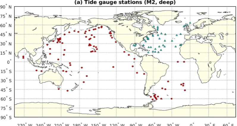
Fig. 12displays the locations of the tide gauge stations in (a) the deep oceans and (b) shallow water (coastal-shelf) regions. For the deep oceans, the tidal data from 132 stations are used for comparison, and 44 out of 132 stations are located in the North Atlantic Ocean (cyan tri-angles). For the shallow water regions, 75 stations of the total 128 sites are located in the North Atlantic Ocean. To check the effect of the two-way nesting on local and remote tides, these stations are divided into two groups: 38 tide gauges along the East Coast of North America (blue squares), and 37 gauges along the European Shelf (cyan triangles). The root-mean-square error between the tide gauge measurements and the HYCOM, TPXO9-atlas, and FES2014 tidal solutions, averaged over all gauges, is evaluated as

= =

N a e a e

RMS 1 1

2 | |

TG k

N

k k

1

ik ik2

(9) wherei= 1,kis the tide gauge station number,Nis the number of the tide gauge stations,a and are the amplitude and phase of the tide gauge data,aandϕare the amplitude and phase of the tidal solutions of

HYCOM, TPXO9-atlas, or FES2014, respectively. The tidal solutions are interpolated onto the locations of the tide gauge stations with a bi-cubic interpolation method.Table 7 shows the gauge-averaged root-mean-square error of the tidal solutions from the tide gauge data in the North Atlantic Ocean (NATL) and the global ocean (GLB) for the TPXO9-atlas and FES2014 tidal solutions, and for the stand-alone 1/25° HYCOM (GLB25) and the two-way nesting results.

The overall surface tidal accuracy is improved through two-way nesting in both the deep oceans and the shallow shelf seas. The im-provement generally decreases farther away from the child domain. The reduction in RMSTGof ∼3 cm is the largest for the North American

East Coast tide gauges, which are located closest to the child domain. For these gauges, the relative improvement of tidal predictability (RMSTG, GLB25− RMSTG, two−way)/RMSTG, GLB25= 15.89%. However,

the two-way nesting reduces the tidal accuracy for the gauges on the European Shelf by 2.22%. The relative improvement of predictability is 8.94% for all the gauges in the deep North Atlantic Ocean, which is larger than the improvement of 6.24% for all the gauges in the deep global ocean. The FES2014 and the TPXO9-atlas solutions have a better tidal accuracy than the HYCOM results. Small differences exist between the FES and TPXO solutions, although FES2014 is generally more ac-curate than TPXO9-atlas in both the deep and shallow oceans, except on the European shelf where the TPXO solution is more accurate.

The tide gauge data set is limited in spatial coverage. Hence, we also validate the global HYCOM simulations with the FES2014 and TPXO9-atlas tidal solutions. At each computational cell (i,j) of HYCOM, we calculate the M2sea-surface-height root-mean-square error between the

HYCOM simulations and the FES/TPXO solutions as (Shriver et al., 2012)

= a e a e

RMSE 1

2 | |

i j, i j, ii j, i j, ii j, 2 ₍₁₀₎

whereaandϕare the amplitude and phase of the M2barotropic tide in

HYCOM, anda and are the amplitude and phase of the global tidal solutions of TPXO9-atlas or FES2014, respectively. Since the HYCOM grid differs from the FES and TPXO grids, the FES2014 and TPXO9-atlas solutions are interpolated onto the HYCOM grid with a bi-cubic inter-polation. Fig. 13a shows the amplitudes and phases of the M2

baro-tropic tide for the two-way nesting simulation. The RMSE between FES2014 and the two-way nesting simulation is depicted inFig. 13b. Fig. 13c shows the improvement of predictability of the global M2 barotropic tide through two-way nesting, ΔRMSE = RMSEGLB25

− RMSEtwo−way. An increase in ΔRMSE through two-way nesting

cor-responds to a reduction in RMSE relative to the reference solution without nesting. The RMSE values of the two-way nesting experiment

and ΔRMSE in the region of the child domain are also plotted inFig. 14. InFigs. 13c and14b, the warm (cool) colors indicate an improvement (reduction) of the predictability through two-way nesting.Figs. 13c and 14b show that the predictability is not only improved in the child do-main, but also in the parent domain outside the child area as far as the South Atlantic Ocean. This clearly illustrates that the improved accu-racy in the coastal-shelf region of the child domain is allowed to pro-pagate to the open ocean through the two-way nesting.

In addition, the spatially averaged root-mean-square error over several ocean domains (RMSavg) is evaluated as (Arbic et al., 2004)

= = =

= =

RMSavg j (RMSE )

N i N

i j i j

j N

i N

i j 1 1 , 2 ,

1 1 ,

j i

j i A

A ₍₁₁₎

Fig. 10.Time-averaged tidal energy flux integrated along the cells parallel to the updated boundary: (a) south, (b) east, (c) north, and (d) west.

Table 6

Specifications for the realistic global-scale case.

Child (HBF) Parent (GLB)

Grid resolution (°) 1/75 1/25

Number of cells 2682 × 7614 9000 × 7055

Number of MPI processes 1408 1296

OASIS3-MCT interpolation Bi-linear Bi-linear

Barotropic time step, ΔtT(s) 1.0 3.0

Baroclinic time step, ΔtC(s) 16.0 48.0

Nesting time step, ΔtNT(s) 3.0 3.0

Excluding zones,Nn,s,e,w(cells) 10 N/A

Smoothing zones,NR(cells) 10 N/A

Low-resolution zones,NB(cells) 10 N/A

Fig. 12.Location of tide gauge stations in the global ocean (GLB) in (a) deep ocean and (b) shallow water. The deep-ocean stations in the North Atlantic Ocean (NATL) are represented by cyan triangles, and the shallow-water stations in NATL are grouped into the western stations (blue squares) and the eastern stations (cyan triangles). The stations in other oceans are shown in red circles for both deep ocean and shallow water. (For interpretation of the references to color in this figure legend, the reader is referred to the web version of this article.)

Table 7

Gauge-averaged M2sea-surface-height root-mean-square error between the tide

gauge data and the tidal solutions (RMSTG, cm). The relative improvement of

tidal predictability is abbreviated with RIOP.

Case NATL GLB

Deep Shallow Deep Shallow

North Am. East Coast Europe

TPXO 0.55 2.23 2.78 0.52 6.18

FES 0.32 1.73 3.30 0.30 3.59

GLB25 8.39 18.06 16.22 5.77 18.94

Two-way 7.64 15.19 16.58 5.41 18.38

Fig. 13.(a) Amplitudes and phases of the M2barotropic tide for the two-way nesting solution, (b) M2sea-surface-height RMSE between FES2014 and the two-way

number of ocean cells in the longitudinal and latitudinal directions, respectively.Table 8represents the root-mean-square error averaged over the child area in the parent domain (HBF), the North Atlantic Ocean (NATL), and the global parent domain (GLB), respectively, for water depths > 5.0 m. In addition, RMSavg is computed over water

depths > 1000 m and latitudes equatorward of 66° (GLB66) for

com-parison with previous studies. The differences in RMSavgcomputed with

either FES2014 or TPXO9-atlas are small. The improvement of pre-dictability is largest in the child domain (7.26%) when TPXO is used. This relative improvement is smaller than the 15.89% improvement computed for the tide gauges on the shelf of the North American East Coast (Table 7). As can be seen inFigs. 12b and14b, these tide gauges are located in areas where ΔRMSE is both large and positive. The re-lative improvement of 7.26% averaged over the child domain is lower due to localized reductions in the predictability in Hudson Bay and Foxe Basin (blue areas inFig. 14b). The improvement in predictability de-creases as the size of the averaging area inde-creases. However, this re-duction in predictability is minimal for the North Atlantic (NATL), where the relative improvement in predictability is 7.03% when FES is used. This relatively large value can be attributed to ΔRMSE being positive over a large area (Fig. 13c). However, beyond the Atlantic Ocean, the improvement in tidal accuracy is minimal. As a con-sequence, the reduction in RMSavgfor the GLB66case is small, i.e., only

2.18%.

While the reduction in RMSE may not seem very large, the surface area where the predictability is improved is generally much larger than the area where it is reduced (Table 9). In the HBF domain, ΔRMSE > 5.0 mm occurs in 64.44% of the domain, while ΔRMSE < − 5.0 mm occurs only in 5.84% of the domain. The largest reduction in

predictability (increase in RMSE) is observed in Foxe Basin (Fig. 14b). In about 1.10% of the North Atlantic Ocean (NATL), the predictability in the two-way nesting solution is reduced. This reduction mostly oc-curs in other shelf regions such as the English Channel, the Patagonian Shelf, and the Amazon Shelf, as shown inFig. 13c. Only 9.69% of the global ocean (GLB) features an improved predictability because the Pacific and Indian Oceans are minimally affected by the two-way nesting in the North Atlantic Ocean.

5. Discussion and conclusions

We have implemented an online two-way nesting framework in a global ocean circulation model (HYCOM) to improve global surface tides. The barotropic pressure and velocity are exchanged between a parent and a child domain with an external coupler, OASIS3-MCT. We modified the masks in both the firstcoarse-to-fineand the second fine-to-coarsedirections, and set the limits of the search area in the first di-rection to reduce the computing time of the remapping coefficients in OASIS3-MCT.

In the global HYCOM simulations, Hudson Strait and the adjacent North Atlantic Ocean feature relatively large M2 sea-surface-height

root-mean-square errors with the tide gauges and the altimetry con-strained tide models. These errors may be associated with the inability of low-resolution simulations to resolve the semi-diurnal tidal re-sonances on and off the shelf in the North Atlantic Ocean. These errors can be reduced by two-way nesting a high-resolution child domain in a low-resolution parent domain. Hence, we selected the Hudson Strait region as the child domain in our nesting experiments.

The developed two-way nesting framework is validated with six semi-idealized one- and two-way nesting experiments. In these Fig. 14.(a) M2sea-surface-height RMSE between FES2014 and the two-way nesting solution and (b) the improvement of predictability in the vicinity of the child

domain. In the figure, thexandyaxes represent the computational indexesiandj, respectively, for a clear view. The corresponding longitudes and latitudes can be found inFig. 11. (For interpretation of the references to color in this figure, the reader is referred to the web version of this article.)

Table 8

Area-averaged root-mean-square error (RMSavg) with TPXO9-atlas (TPXO) and

FES2014 (FES) for four areas of GLB25 (1/25° simulation without nesting) and two-way nesting solutions (cm). The relative improvement of tidal predict-ability is abbreviated with RIOP.

Case HBF NATL GLB GLB66

TPXO FES TPXO FES TPXO FES TPXO FES

GLB25 20.57 18.45 9.61 8.68 6.67 5.93 4.13 4.12

2-way 19.18 17.11 9.08 8.07 6.60 5.85 4.05 4.03

RIOP 6.76% 7.26% 5.52% 7.03% 1.05% 1.35% 1.94% 2.18%

Table 9

Area integral over ocean surface where ΔRMSE > 5 mm (improved predict-ability) and ΔRMSE < − 5 mm (reduced predictpredict-ability) with FES2014 for the child domain (HBF), the North Atlantic (NATL), and the global ocean (GLB). The fraction of the total area is between parentheses.

RMSE reduction (×104_km2_{) HBF NATL GLB}

ΔRMSE > 5 mm (improvement) 321.95 2271.62 3456.01

(64.44%) (49.83%) (9.69%)

ΔRMSE < − 5 mm (reduction) 29.20 49.93 550.03

experiments, the child domain covers the Hudson Strait region, while the parent domain covers the Arctic, North Pacific, and North Atlantic Oceans. The M2barotropic tide is forced at the southern boundary of

the parent domain. The accuracy of the nesting framework is tested for time steps and grid resolutions that are the same and/or differ between the parent and child domains. The parent and child grids have the same resolution in Experiments 1–4. The tidal solution on the parent grid without nesting is used as the ‘true’ reference solution. The semi-idea-lized experiments have a good agreement with the reference solution. The errors of the sea-surface height in the four experiments are gen-erally much < 1%. In addition, two experiments are performed in which the grid resolution of the child domain is three times as fine (1/ 75°) as that of the parent domain (1/25°) to check for discontinuities along the nesting boundaries. It is shown that mass and energy are conserved across the boundaries through all the experiments.

Next, the developed two-way nesting framework is applied to a realistic global-scale experiment. The resolution of the child domain (1/ 75°) is three times as high as that of the parent domain (1/25°). Realistic tidal forcing (M2, S2, N2, K1, and O1) and atmospheric pressure

(MSLP) are applied over the child domain (HBF) as well as the parent domain (GLB). Compared to the child domain of the semi-idealized experiments, the HBF domain is extended to Hudson Bay and the Bay of Fundy to improve the tidal accuracy in these areas. The no-nesting and two-way nesting results are compared to tide gauge data and the FES2014 and TPXO9-atlas tidal solutions. The application of the two-way nesting reduces the M2sea-surface-height root-mean-square errors

with the tide gauge data and the tidal solutions, in particular in the Northwest Atlantic Ocean. The largest improvement of predictability (i.e., reduction of the root-mean-square error) of about 16% occurs at the tide gauges located along the East Coast of North America. The M2

root-mean-square errors between the two-way nesting simulation and the TPXO/FES tidal solutions are not only reduced in the vicinity of the child domain, but they are reduced as far as the South Atlantic Ocean (red areas in Figs. 13c and 14b). The improvement of the tidal pre-dictability in the North Atlantic Ocean averages about 6.28%. The two-way nesting simulation shows that a higher horizontal grid resolution and a better resolved coastal bathymetry in the regions of Hudson Strait and the Bay of Fundy not only improves the tidal prediction in the child domain, but also in the coastal and abyssal ocean away from the nesting boundaries through the back-effect (Arbic and Garrett, 2010; Arbic et al., 2009;Arbic et al., 2007).

In recent years, the global-mean M2sea-surface-height

root-mean-square error between 1/12.5°_{HYCOM and TPXO tidal solutions has}

been reduced from 7.48 cm in Shriver et al. (2012) to 4.43 cm in Buijsman et al. (2015)to 2.60 cm in Ngodock et al. (2016). The re-duction from 7.48 cm to 4.43 cm is due to the inclusion of bathymetry under the ice shelves, the application of a spatially varying and iterated SAL, and the tuning of the linear wave drag. The reduction from 4.43 cm to 2.60 cm is due to the application of an augmented state ensemble Kalman Filter (ASEnKF) to correct for errors in the tide model asso-ciated with imperfectly known topography and damping terms. In this paper, we do not apply the ASEnKF technique. The reduction in RMSE from 4.43 cm to 4.13 cm for the no-nesting solution is due to an in-crease in model resolution from 1/12.5°_{to 1/25}°_{. The application of the}

two-way nesting framework to one area, i.e. the Hudson Shelf, reduces this global-mean error to 4.03 cm, which is a modest improvement.

This paper mainly describes the development of a two-way nesting framework in a non-data-assimilative version of HYCOM and its vali-dation with the tide gauge data and the global FES2014 and TPXO9-atlas tidal solutions. To reduce the large M2surface tide errors in the

North Atlantic, a high resolution child grid is applied to the Hudson Shelf. This improves the accuracy of the tides not only in the Hudson Shelf region, but also in the Atlantic Ocean as far south as South Africa. However, the European Shelf, the Patagonian Shelf, and the Northwest Australian Shelf, among others, still feature large sea-surface-height root-mean-square errors in HYCOM (Fig. 13b). To further reduce these

errors, we plan to apply the two-way nesting technique to multiple shelf areas in different ocean basins and find the break-even point where two-way nesting is computationally efficient compared to the stand-alone high-resolution global simulation in a subsequent paper.

Acknowledgment

C.-H.J., M.C.B., B.K.A., and J.G.R. gratefully acknowledge funding from the project “Improving global surface and internal tides through two-way coupling with high resolution coastal models” as part of the Office of Naval Research (ONR) grant N00014-15-1-2288. A.J.W. and J.F.S. acknowledge support from the Naval Research Laboratory (NRL) contract N00014-15-WX-01744. Finally, P.J.H. acknowledges financial support from the project “Arctic shelf and large rivers seamless nesting in global HYCOM” as part of ONR grant N00014-15-1-2594.

References

Arbic, B.K., Garrett, C., 2010. A coupled oscillator model of shelf and ocean tides. Cont. Shelf Res. 30, 564–574.https://doi.org/10.1016/j.csr.2009.07.008.

Arbic, B.K., Garner, S.T., Hallberg, R.W., Simmons, H.L., 2004. The accuracy of surface elevations in forward global barotropic and baroclinic tide models. Deep-Sea Res. II 51, 3069–3101.https://doi.org/10.1016/j.dsr2.2004.09.014.

Arbic, B.K., St-Laurent, P., Sutherland, G., Garrett, C., 2007. On the resonance and in-fluence of the tides in Ungava Bay and Hudson Strait. Geophys. Res. Lett. 34, L17606.

https://doi.org/10.1029/2007GL030845.

Arbic, B.K., Karsten, R.H., Garrett, C., 2009. On tidal resonance in the global ocean and the back-effect of coastal tides upon open-ocean tides. Atmosphere-Ocean 47, 239–266.https://doi.org/10.3137/OC311.2009.

Arbic, B.K., Wallcraft, A.J., Metzger, E.J., 2010. Concurrent simulation of the eddying general circulation and tides in a global ocean model. Ocean Model 32, 175–187.

https://doi.org/10.1016/j.ocemod.2010.01.007.

Barth, A., Alvera-Azcárate, A., Rixen, M., Beckers, J.M., 2005. Two-way nested model of mesoscale circulation features in the Ligurian Sea. Prog. Oceanogr. 66, 171–189.

https://doi.org/10.1016/j.pocean.2004.07.017.

Bleck, R., Smith, L.T., 1990. A wind-driven isopycnic coordinate model of the North and Equatorial Atlantic Ocean: 1. Model development and supporting experiments. J. Geophys. Res. 95, 3273–3285.

Bowden, J.H., Otte, T.L., Nolte, C.G., Otte, M.J., 2012. Examining interior grid nudging techniques using two-way nesting in the WRF model for regional climate modeling. J. Clim. 25, 2805–2823.https://doi.org/10.1175/JCLI-D-11-00167.1.

Browning, G., Kreiss, H.O., 1982. Initialization of the shallow water equations with open boundaries by the bounded derivative method. Tellus 34, 334–351.

Buijsman, M.C., Arbic, B.K., Green, J.A.M., Helber, R.W., Richman, J.G., Shriver, J.F., Timko, P.G., Wallcraft, A., 2015. Optimizing internal wave drag in a forward baro-tropic model with semidiurnal tides. Ocean Model 85, 42–55.https://doi.org/10. 1016/j.ocemod.2014.11.003.

Cancet, M., Andersen, O.B., Lyard, F., Cotton, D., Benveniste, J., 2018. Arctide2017, a high-resolution regional tidal model in the Arctic Ocean. Adv. Space Res. 62, 1324–1343.https://doi.org/10.1016/j.asr.2018.01.007.

Carrère, L., Lyard, F., Cancet, M., Guilot, A., 2015. FES2014, a New Tidal Moel on the Global Ocean with Enhanced Accuracy in Shallow Seas and in the Arctic Region, EGU General Assembly 2015, Vienna, Austria, 12–17 April, 5481.

Chassignet, E.P., Hurlburt, H.E., Smedstad, O.M., Halliwell, G.R., Hogan, P.J., Wallcraft, A.J., Baraille, R., Bleck, R., 2007. The HYCOM (HYbrid Coordinate Ocean Model) data assimilative system. J. Mar. Syst. 65, 60–83.https://doi.org/10.1016/j.jmarsys. 2005.09.016.

Debreu, L., Blayo, E., 2008. Two-way embedding algorithms: a review. Ocean Dyn. 58, 415–428.https://doi.org/10.1007/s10236-008-0150-9.

Debreu, L., Marchesiello, P., Penven, P., Cambon, G., 2012. Two-way nesting in split-explicit ocean models: algorithms, implementation and validation. Ocean Model 49-50, 1–21.https://doi.org/10.1016/j.ocemod.2012.03.003.

Defant, A., 1961. Physical Oceanography. Pergamon Press, Oxford.

Egbert, G.D., Erofeeva, S.Y., 2002. Efficient inverse modeling of barotropic ocean tides. J. Atmos. Ocean. Technol. 19, 183204.https://doi.org/10.1175/1520-0426(2002) 019<0183:EIMOBO>2.0.CO;2.

Egbert, G.D., Ray, R.D., 2001. Estimates of M2 tidal energy dissipation from Topex/ Poseidon altimetry data. J. Geophys. Res. 106, 475–502.

Egbert, G.D., Ray, R.D., Bills, B.G., 2004. Numerical modeling of the global semidiurnal tide in the present day and in the Last Glacial Maximum. J. Geophys. Res. 109, C03003.https://doi.org/10.1029/2003JC001973.

Fox, A.D., Maskell, S.J., 1995. Two-way interactive nesting of primitive equation ocean models with topography. J. Phys. Oceanogr. 25, 2977–2996.

Ginis, I., Richardson, R.A., Rothstein, L.M., 1998. Design of a multiply nested primitive equation ocean model. Mon. Weather Rev. 126, 1054–1079.

Green, J.A.M., Nycander, J., 2013. A comparison of tidal conversion parameterizations for tidal models. J. Phys. Oceanogr. 43, 104–119. https://doi.org/10.1175/JPO-D-12-023.1.

assimilation system”. Ocean Dyn. 60, 1497–1537. https://doi.org/10.1007/s10236-010-0349-4.

Herrnstein, A., Wickett, M., Rodrigue, G., 2005. Structured adaptive mesh refinement using leapfrog time integration on a staggered grid for ocean models. Ocean Model 9, 283–304.https://doi.org/10.1016/j.ocemod.2004.07.002.

Hogan, P.J., Hurlburt, H.E., 2006. Why do intrathermocline eddies form in the Japan/ East Sea? Oceanography 19, 134–143.

Hogan, T.F., Liu, M., Ridout, J.A., Peng, M.S., Whitcomb, T.R., Ruston, B.C., Reynolds, C.A., Eckermann, S.D., Moskaitis, J.R., Baker, N.L., McCormack, J.P., Viner, K.C., McLay, J.G., Flatau, M.K., Xu, L., Chen, C., Chang, S.W., 2014. The navy global en-vironmental model. Oceanography 27, 116–125.

Juricke, S., Goessling, H.F., Jung, T., 2014. Potential sea ice predictability and the role of stochastic sea ice strength perturbations. Geophys. Res. Lett. 8396–8403.https://doi. org/10.1002/2014GL062081.

Lam, F.P.A., Haley Jr., P.J., Janmaat, J., Lermusiaux, P.F.J., Leslie, W.G., Schouten, M.W., te Raa, L.A., Rixen, M., 2009. At-sea real-time coupled four-dimensional oceano-graphic and acoustic forecasts during Battlespace Preparation 2007. J. Mar. Syst. 78, S306–S320.https://doi.org/10.1016/j.jmarsys.2009.01.029.

Ličer, M., Smerkol, P., Fettich, A., Ravdas, M., Papapostolou, A., Mantziafou, A., Strajnar, B., Cedilnik, J., Jeromel, M., Jerman, J., Petan, S., Malačič, V., Sofianos, S., 2016. Modeling the ocean and atmosphere during an extreme bora event in northern Adriatic using one-way and two-way atmosphere-ocean coupling. Ocean Sci. 12, 71–86.https://doi.org/10.5194/os-12-71-2016.

Lorenz, P., Jacob, D., 2005. Influence of regional scale information on the global circu-lation: a two-way nesting climate simulation. Geophys. Res. Lett. 32, L18706.https:// doi.org/10.1029/2005GL023351.

Mason, E., Molemaker, J., Shchepetkin, A.F., Colas, F., McWilliams, J.C., 2010. Procedures for offline grid nesting in regional ocean models. Ocean Model 35, 1–15.

https://doi.org/10.1016/j.ocemod.2010.05.007.

Metzger, E.J., Hurlburt, H.E., Xu, X., Shriver, J.F., Gordon, A.L., Sprintall, J., Susanto, R.D., van Aken, H.M., 2010. Simulated and observed circulation in the Indonesian seas: 1/12° global HYCOM and the INSTANT observation. Dyn. Atmos. Oceans 50, 275–300.https://doi.org/10.1016/j.dynatmoce.2010.04.002.

Ngodock, H.E., Souopgui, I., Wallcraft, A.J., Richman, J.G., Shriver, J.F., Arbic, B.K., 2016. On improving the accuracy of the M2barotropic tides embedded in a

high-resolution global ocean circulation model. Ocean Model 97, 16–26.https://doi.org/ 10.1016/j.ocemod.2015.10.011.

Penven, P., Debreu, L., Marchesiello, P., McWilliams, J.C., 2006. Evaluation and appli-cation of the ROMS 1-way embedding procedure to the central California upwelling system. Ocean Model 12, 157–187.https://doi.org/10.1016/j.ocemod.2005.05.002. Qi, J., Chen, C., Beardsley, R.C., 2018. FVCOM one-way and two-way nesting using ESMF:

development and validation. Ocean Model 124, 94–110.https://doi.org/10.1016/j. ocemod.2018.02.007.

Santilli, E., Scotti, A., 2015. The stratified ocean model with adaptive refinement. J. Comput. Phys. 291, 60–81.https://doi.org/10.1016/j.jcp.2015.03.008.

Shriver, J.F., Arbic, B.K., Richman, J.G., Ray, R.D., Metzger, E.J., Wallcraft, A.J., Timko, P.G., 2012. An evaluation of the barotropic and internal tides in a high-resolution global ocean circulation model. J. Geophys. Res. 117, C10024.https://doi.org/10. 1029/2012JC008170.

Spall, M.A., Holland, W.R., 1991. A nested primitive equation model for oceanic appli-cations. J. Phys. Oceanogr. 21, 205–220.

Stammer, D., Ray, R.D., Andersen, O.B., Arbic, B.K., Bosch, W., Carrère, L., Cheng, Y., Chinn, D.S., Dushaw, B.D., Egbert, G.D., Erofeeva, S.Y., Fork, H.S., Green, J.A.M., Griffiths, S., King, M.A., Lapin, V., Lemoine, F.G., Luthcke, S.B., Lyard, F., Morison, J., Müller, M., Padman, L., Richman, J.G., Shriver, J.F., Shum, C.K., Taguchi, E., Yi, Y., 2014. Accuracy assessment of global barotropic ocean tide models. Rev. Geophys. 52, 243–282.https://doi.org/10.1002/2014RG000450.

Tang, H.S., Qu, K., Wu, X.G., 2014. An overset grid method for integration of fully 3D fluid dynamics and geophysics fluid dynamics models to simulate multiphysics coastal ocean flows. J. Comput. Phys. 273, 548–571.https://doi.org/10.1016/j.jcp. 2014.05.010.

Urrego-Blanco, J., Sheng, J., Dupont, F., 2016. Performance of one-way and two-way nesting techniques using the shelf circulation modelling system for the Eastern Canadian Shelf. Atmosphere-Ocean 54, 75–92.https://doi.org/10.1080/07055900. 2015.1130122.

Valcke, S., Balaji, V., Craig, A., DeLuca, C., Dunlap, R., Ford, R., Jacob, R., Larson, J., O'Kuinghttons, R., Riley, G., Vertenstein, M., 2012. Coupling technologies for earth system modelling. Geosci. Model Dev. 5, 1589–1596. https://doi.org/10.5194/gmd-5-1589-2012.

Valcke, S., Craig, T., Coquart, L., 2015. OASIS3-MCT User Guide. Technical Report TR/ CMGC/15/38. CERFACS/CNRS SUC URA, Toulouse, France.

Wahle, K., Staneva, J., Koch, W., Fenoglio-Marc, L., Ho-Hagemann, H.T.M., Stanev, E.V., 2017. An atmosphere-wave regional coupled model: improving predictions of wave heights and surface winds in the southern North Sea. Ocean Sci. 13, 289–301.

https://doi.org/10.5194/os-13-289-2017.

Will, A., Akhtar, N., Brauch, J., Breil, M., Davin, E., Ho-Hagemann, H.T.M., Maisonnave, E., Thürkow, M., Weiher, S., 2017. The COSMO-CLM 4.8 regional climate model coupled to regional ocean, land surface and global earth system models using OASIS3-MCT: description and performance. Geosci. Model Dev. 10, 1549–1586.

https://doi.org/10.5194/gmd-10-1549-2017.