The continuity and estimates of a solution to mixed fractional constant elasticity of variance system with stochastic volatility and the pricing of vulnerable options

R E S E A R C H

Open Access

The continuity and estimates of a solution to

mixed fractional constant elasticity of

variance system with stochastic volatility and

the pricing of vulnerable options

Yan Dong

*_{Correspondence:} dongyan840214@126.com 1_{Department of Basic, Shaanxi}

Railway Institute, Weinan, China

Abstract

Stochastic volatility models play an important role in finance modeling. Under a mixed fractional Brownian motion environment, we study the continuity and estimates of a solution to a kind of stochastic differential equations with double volatility terms. Besides, we propose to price the vulnerable option with the discretization method and present the results using a Monte Carlo simulation.

MSC: 35K99; 97M30

Keywords: Mixed fractional constant elasticity of variance model; Strong solution; Existence; Uniqueness; Continuity

1 Introduction

Most of the existing literature on financial models assumes that the volatility of assets is constant. However, this assumption ignores the return features of volatility clustering, high peak, fat tails, and volatility mean reverting in real markets, which cannot be captured by constant volatility models [1,2]. To model the volatility smile effectively, one solution is using the stochastic volatility under two cases: (1) the function of stochastic processes is used to describe the volatility [3,4], and (2) the additional Brownian motion is introduced to describe the stochastic parts of stochastic volatility (SV) models. In this paper, we focus on the second case.

Stochastic volatility models constituted of one stock have been introduced and inten-sively investigated in the literature. Hull and White [5] first introduce an SV model called the Heston model in which the market volatility follows a mean-reverting Cox–Ingersoll– Ross process. Starting with Xu and Taylor [6], lots of studies show that two-component volatility models outperform one-component ones in the option pricing literature (see [7,8]). Da Fonseca et al. [9] extend the Heston model to a multifactor specification for the volatility process in a single asset framework. Wang et al. [10] extend the framework of Siu et al. [11] and focus on currency options under a two-factor Markov-modulated stochastic volatility jump-diffusion model. The theoretical development of the SV model

is introduced in [12] by studying the following equations:

⎧ ⎨ ⎩

dS(t) =rS(t) dt+√v(t)S(t) dB1(t),

dv(t) =κ(θ–v(t)) dt+σ(v(t)) dB2(t),

(1.1)

where time variablet∈(0,T),B1(t) andB2(t) are mutually independent standard

Brown-ian motions, andr> 0 is the constant risk-free interest rate. Herev(t) is a mean-reverting square-root process, whereasκ> 0 specifies the speed of adjustment of the volatility to-ward its theoretical meanθ> 0. Note thatσ> 0 is the second-order volatility, that is, the volatility of volatility. The paper [12] also studies the existence and uniqueness of a strong solution to (1.1). CertainLp_{estimates of (1.1) are proved in [13].}

However, all the existing SV models mentioned are based on the Brownian motion with increments following theindependent normdistribution. Many works argue that the re-turns of risky assets have long-range dependence properties, which are expressed by the increment of financial models. Using the Brownian motion to express the stochastic parts without considering its dependency to the financial modeling may have some serious dis-advantages [14]. Because of the self-similarity and long-range dependence properties, the fractional Brownian motion becomes a suitable tool in mathematical finance. We refer the readers to [14,15] for the motivation and references concerning the study of the fractional Brownian motion.

It is worth noting that the SV models shown in the above references constitute one stock. Thus those SV models cannot be used to study vulnerable option shown in Sect.5, because the vulnerable option is constructed by two stocks.

In this paper, we use the mixed fractional Brownian motion (mfBm), which is a linear combination of a Brownian motion and fractional Brownian motion, to drive the following stock price systems constituted of two stocks:

⎧ ⎨ ⎩

dS1(t) =rS1(t) dt+ √

V1(t)S1(t)α1dM1,1H(t), S1(0) =s1,

dS2(t) =rS2(t) dt+ √

V2(t)S2(t)α2dM1,2H(t), S2(0) =s2,

(1.2)

where the variance processes{v1(t),t≥0}and{v2(t),t≥0}are driven by the fractional

Cox–Ingersoll–Ross model satisfying

⎧ ⎨ ⎩

dV1(t) =κ1(θ1–V1(t)) dt+σ1

|V1(t)|dM2,1H(t), V1(0) =v1,

dV2(t) =κ2(θ2–V2(t)) dt+σ2

|V2(t)|dM2,2H(t), V2(0) =v2,

(1.3)

dMH_1,1(t)·dMH_1,2(t) = dMH_2,1(t)·dMH_2,2(t) =ρdt2H+λ2dt. (1.4) HereMH

1,1(t),MH1,2(t),M2,1H(t) andM2,2H(t) aremfBmprocesses, which, together with relative

conclusions, will be defined in Sect.2, andαis an elastic constant. We call this model a mixed factional CEV model. It is not an easy task to show that the solutions toV1(t) and

V2(t) are positive whenSVmodel is driven bymfBmprocesses. Thus we use|V1(t)|and |V2(t)|in (1.3) instead ofV1(t) andV2(t) as in the classicalSVmodel.

Sect.4, we price the European option using the discrete type of (1.2)–(1.4) and Monte Carlo simulations.

2 Preliminaries

The mixed fractional Brownian motion is a stochastic process with long memory and plays an important role in the financial modeling. To better understand the rest of the paper, we briefly review some basic concepts and properties of the mixed fractional Brownian motion.

LetHbe a constant belonging to (0, 1). A fractional Brownian motion (fBm){BH_(t),t≥

0}with Hurst parameterHis a continuous and centered Gaussian process with covariance [16]

R(t,s) =EBH(t)BH(s) =1 2

t2H+s2H–|t–s|2H=

t

0

s

0

φ(r,u) dudr

fors,t> 0, whereφ(r,u) =H(2H– 1)|r–u|2H–2. WhenH=1₂, thefBmbecomes a standard Brownian motion denoted by{B(t),t≥0}. A mixed fractional Brownian motion (mfBm)

{MH_{(t),t≥0}is a linear combination of a Brownian motion (Bm) and a fractional}

Brow-nian motion, defined on a filtered probability space (Ω,F,Ft,P) by

MH(t) =λB(t) +BH(t),

whereλis a real constant,Pis a physical probability measure, and{Ft,t≥0}denotes the

P-completion of the filtration generated by (B(t),BH_{(t)). AnmfBm{M}H_{(t),t≥0}has the}

following properties [12,13]

1. MH(0) = 0andE[MH(t)] = 0for anyt≥0.

2. MH_{(t)is a centered Gaussian process, not a Markovian one for allH∈(0, 1).}

3. {MH_{(t),t≥0}has homogeneous increments, that is, the increment}

MH_{(t+s) –M}H_{(s)has the same distribution asB}H_{(t)fors,t≥0.}

4. The covariance ofMH_(t)andMH_{(s)is given by}

EMH(t)MH(s) =λ2·s∧t+R(t,s) fors,t> 0.

5. The increments ofMH_{(t)are positively correlated if0.5 <H< 1, uncorrelated if}

H= 0.5, and negatively correlated if0 <H< 0.5.

At the end of this section, we give some notations, function spaces, and conclusions to prove our main results (for details, see [13–15]).

LetS(R) be the Schwartz space of rapidly decreasing smooth functions onRwith norm

f2_H=

R

R

f(s)f(t)φ(s,t) dsdt<∞.

If we equipS(R) with the inner product

f,g H=

R

R

f(s)f(t)φ(s,t) dsdt<∞,

Recall that anmfBmis a linear combination of aBmandfBm. The stochastic integral with respect to aBm has been studied by many references. We present the fractional Wick–Itô–Skorokhod (fWIS) integral theory.

The stochastic integral with respect tofBmfor deterministic functions is easily defined.

Lemma 2.1 If f,g belong to L2

H(R),then

Rf(s) dBHs and

Rg(s) dBHs are well-defined

zero-mean Gaussian random variables with variancesf2

Handg2H,respectively,and

E

R

f(s) dBH_s

R

g(s) dBH_s

=f,g H.

Proof This lemma is verified in [16]. It can be directly proved by verifying it for simple functionsn_i=1aiI(ti,ti+1]and then proceeding with a passage to the limit. Definition 2.1 SupposeY: R→(S)∗_H is a given function such thatY(t)♦W(H)_{(t) is}

dt-integrable in (S)∗_H. Then we define its fractional Wick–Itô–Skorokhod (fWIS) integral

RY(t) dBHt by

R

Y(t) dBH_t =

R

Y(t)♦W(H)(t) dt.

In particular, the integral on an interval can be defined as

T

0

Y(t) dBH_t =

R

Y(t)I[0,T]dBHt .

Here (S)∗_His the fractional Hida distribution space, and♦stands for the Wick product (for details, see [16]).

Example2.1 SupposeY(t) is a step functionY(t) =n_i=1Fi(ω)I[ti,ti+1)(t), where the random

variablesFi(ω)∈(S)∗H, and a partitionπsatisfies 0 =t0<t1<· · ·<tn=T. Then

T

0

Y(t) dBH_t =

n

i=1

Fi(ω)♦

BH_ti+1–BH_ti.

LetLp_(PH_{) =L}p_{be the space of all random variablesF:Ω→R such that} FLp_(PH₎=E

|F|p 1/p<∞.

Definition 2.2 Letg∈L2

H(R). Theφ-derivative of a random variableF∈Lp(PH) in the

direction ofΦgis defined as

DΦgF(ω) =lim δ→0

1

δ

F

ω+δ

·

0

(Φg)(u) du

–F(ω)

,

provided that the limit exists inLp_(PH_{). Furthermore, if there is a process (D}φ

sF,s> 0) such

that

DΦgF=

R

Dφ

sFgsds almost surely

Lemma 2.2 If g∈L2

H(R),F∈L2(PH),and DΦgF∈L2(PH),then

F♦

R

gsdB(H)s =F

R

gsdB(H)s –DΦgF.

3 Moment estimates

In this section, we prove moment estimates and continuity of the solution of the mixed fractional CEV system (1.2)–(1.3) by extending the idea of [13] for a mixed stochastic differential equation.

Lemma 3.1 If X obeys the normal distribution with zero mean,then for any constant p≥1,

there exists a constant c1(p),depending only on p,such that

E|X|p ≤c1(p)E

|X| p. (3.1)

Proof LetX∼N(0,σ2) andf(x) =_√1

2π σ2exp{–x 2

2σ2}. Ifn≥2 is an even number, then it is

easy to have

E|X|n = 2

+∞

0

xnf(x) dx=√ 2 2π σ2

+∞

0

xnexp

– x 2σ2

dx.

Usingt=_2σx2, we have

E|X|n = 2

+∞

0

xnf(x) dx=(

√

2)n

√

π σ n

+∞

0

tn–12 _exp{_–t}_dx.

Recall thatΓ(n) =₀+∞tn–1_{exp{–t}dx, Thus we useΓ(n) = (n– 1)Γ(n– 1) andΓ(0.5) =} √

πto arrive at

E|X|n = 2

+∞

0

xnf(x) dx=(

√

2)n

√

π σ n_Γ

n+ 1

2

= (n– 1)!σn. (3.2)

Letp≥1 be a positive constant. We define

n=min{m|p≤m,mis an even number}.

Using the Hölder inequality and combining (3.2), we obtain

E|X|p ≤E|X|n

p

n_{= (n)!}p_n·σp_{. (3.3)}

Now we focus onE[|X|]. A change of variable for integral gives

E|X| = 2

R

xf(x) dx=√2 2π σ

R

xexp

– x

2

2σ2

dx

=√1 2π σ

R

exp

– x

2

2σ2

Lettingt=₂x_σ22 and using integration by substitution, we have

E|X| =√2/π·σ

R

exp{–t}dt=σ√2/π. (3.4)

Combining (3.2), (3.3), and (3.4), the lemma is proved.

Lemma 3.2 If V1(t)is the solution of volatility equation(1.3),then for any p≥2,we have

E t

0

V1(s)dBHs

p≤c2(p,H)Hp2p–1

T

0

EV1(t) p

dt+c3(p,H,T),

where c2(p,H) =1₂c1(p)Hpand c3(p,H,T) = ₂1pc(p)Hp2p–1(

T

0 t2H–2dt)p.

Proof For a partitionπ: 0 =t0<t1<· · ·<tn=t, let

S|V1|,π

= n–1 i=0

V1(t)♦

B(H)ti+1–B

(H) ti

. (3.5)

According to the WIS integral with respect to fBm, we have

t

0

V1(s)dB(H)s =_|πlim_|→ 0S

|V1|,π

. (3.6)

Note that, for fixedti,V1(ti) is a random variable. Using (3.37) in [15], we have

V1(ti)♦

B(H)ti+1–B

(H) ti

=V1(t)·

R

I(ti,ti+1]dB

(H) s –D

φ Φg

V1(ti)

=V1(t)·

R

I(ti,ti+1]dB

(H) s =

V1(t)·

B(H)ti+1–B

(H) ti

. (3.7)

Substituting (3.7) into (3.5) and using the triangle and Hölder inequalities, we obtain

ES|V1|,π ≤ n–1

i=0

EV1(t)·

B(H)ti+1–B

(H) ti ≤ n–1 i=0

EV1(t) ·EB(H)ti+1–B

(H) ti

2

. (3.8)

Letting|π| →0 and combining (3.6) and (3.8), we obtain

E t

0

V1(s)dBHs

≤

T

0

EV1(t) dtH.

Using Lemma3.1, we arrive at

E t

0

V1(s)dBHs

≤c1(p)E

t

0

V1(s)dBHs

p≤c1(p)

T

0

EV1(t) dtH

p

. (3.9)

Using the Hölder inequality twice, we have

E t

0

V1(s)dBHs

p≤c1(p)Hp

T

0

1

2EV1(t) + 1 2t

2H–2_dt

p

≤ 1

2pc1(p)H p

T

0

EV1(t) dt+

T

0

t2H–2dt p

.

Using the inequality (a+b)p≤2p–1(ap+bp), we get

E t

0

V1(s)dBHs

p

≤ 1

2pc1(p)H p₂p–1

T

0

EV1(t) dt

p

+

T

0

t2H–2dt p

. (3.10)

Recalling that H ∈(0.5, 1), we have 2H – 2 ∈ (–1, 0). This implies that the integral

T 0 t

2H–2_{dtis convergent. Hence the lemma is proved applying the Hölder inequality to}

(3.10).

Theorem 3.1 Let T> 0be fixed.For p≥2,there are constants c4and c5,depending onλ,

p,σi,κi,H,vi,T,such that

E sup

t∈[0,T]

Vi(t) p

≤ci+3, i= 1, 2.

Proof Here we only prove the casei= 1. Since for anyt∈[0,T],

V1(t) =v1+

t

0 κ1

θ1–V1(s)

ds+σ1

t

0

V1(s)dM2,1H(s),

using the Young inequality, we have for anyp≥2 that

V1(t) p

≤3p–1|v1|p+A1+A2

, (3.11)

whereA1=κ1p|

t

0θ–V1(s) ds|p,A2=σ p 1|

t 0

|V1(s)|dMH2,1(s)|p.

Now, we computeE[A1] andE[A2]. For the second termA1in (3.11), using the Hölder

and Young inequalities, we have

E[A1]≤2p–1κ1pθpT+ 2p–1κ p 1

t

0

V1(s) ds

p

≤2p–1κ₁pθpT+ 2p–1κ₁pTp–1 t

0

EV1(s) p

ds. (3.12)

Noting thatMH

t =λB(t) +BH(t) and applying the inequality (a+b)n≤2n–1(an+bn) toA2,

we have

where A3=|

t 0

|V1(s)|dB(s)|p and A4 =|

t 0

|V1(s)|dBH(s)|p. Applying the B-D-G

in-equality [13,15] toE[A3] and using the inequalityx≤1 +x2, we have

E[A3]≤

t

0

EV1(s) ds

p/2≤

t

0

EV1(s) ds

p+ 1.

Using the Hölder inequality, we obtain

E[A3]≤

t

0

EV1(s) p

ds+ 1. (3.14)

Substituting (3.14) and Lemma3.2into (3.13), we have

E[A2]≤c6(λ,p,σ,T,H)

t

0

EV1(s) p

ds+c7(λ,p,σ1,H,T), (3.15)

where

c6(λ,p,σ,T,H) = 2p–1λpσ1p+ 2p–1λpσ p

1Hpc2(p,H),

c7(λ,p,σ1,H,T) = 2p–1σ1pλp+2p–1λpσ p

1c3(p,H,T).

Substituting (3.12) and (3.15) into (3.11) and letting

c8= 3p–1|v1|p+ 6p–1κ1pθpT+ 3p–1c7(λ,p,σ1,H,T),

c9= 6p–1κ1pTp–1+ 3p–1c6(λ,p,σ1,T,H),

we obtain

EV1(t) p

≤c8+c9

t

0

EV1(s) p

) ds. (3.16)

Hence the theorem follows from the Gronwall inequality.

Lemma 3.3 The claim of Theorem3.1still holds if p∈(0, 2).

Proof If 1≤p< 2, then applying the Cauchy inequality toV1(t) in Theorem3.1, we have

EV1(t) p

≤EV1(t) 2p 1₂

≤ sup

t∈[0,T]

EV1(t) 2p 12

.

Noting that 2p≥2 and using (3.9), we obtain

EV1(t) p

≤C4(λ,p,σ1,θ1,κ1,H,v1,T).

Becauset∈[0,T] is arbitrary, (3.9) is proved for 1≤p< 2. For 0 <p< 1, note that

V1(t) p

=V1(t) p

I{|V1(t)|≥1}+v1(t)

p

≤V1(t) p+1

I{|V1(t)|≥1}+V1(t)

p

I{|V1(t)|<1}.

Further we have

V1(t) p

≤V1(t) p+1

I{|V1(t)|≥1}+ 1≤V1(t)

p+1

+ 1. Hence it follows that, in the case 1 <p< 2,

sup

t∈[0,T]

EV1(t) p

≤c4(λ,p,σ1,θ1,κ1,H,v1,T) + 1.

Thus the proof of the lemma is completed.

Lemma 3.4 The stock price equation of the CEV model has a unique solution.For any positive constant p,we have

sup

t∈[0,T]

ESi(t) p

≤c10(r,λ,p,σi,H,θi,κi,vi,si,T), i= 1, 2. (3.17)

Proof A similar proof of the existence and uniqueness of stock price equation can be found in [14]; (3.17) can be obtained by following the proof of Lemma3.1.

4 Continuous dependence

In this section, we discuss the continuity of the stock price equation of the CEV model.

Theorem 4.1 The stock price process of the CEV model{Si(t),t≥0} is continuous in t,

i= 1, 2.

Proof We only prove the casei= 1. Note that, for any 0≤s<t≤T,

S1(t) –S1(s) =

t

s

rS1(τ) dτ+

t

s

v1(τ)S1(τ)α1dMH1,1(τ).

Using the inequality (a+b)p_≤2p–1_(ap_+bp_{), we obtain}

S(t) –S(s)p≤2p–1A5+ 2p–1A6, (4.1)

whereA5=|

t

srS1(τ) dτ| p_,A

6=|

t s

|v1(τ)|S1(τ)α1dMH1,1(τ)|p. Letp> 0,q> 0, 1p+ 1 q= 1.

Using the Hölder inequality, sincep_q=p– 1, we have

_stS1(τ) dτ

p≤(t–s)pq

t

s

S1(τ)pdτ≤(t–s)p–1

t

s

S1(τ)pdτ. (4.2)

Inequalities (3.17) and (4.2) imply that

E[A5]≤rpc10(r,λ,p,σ1,H,θ1,κ1,v1,s1,T)· |t–s|p. (4.3)

Now we pay attention toE[A6]. By the inequality (a+b)p≤2p–1(ap+bp) we have

A6≤2p–1

t

s

v1(τ)S1(τ)α1dB1,1(τ)

+ 2p–1

t

s

v1(τ)S1(τ)α1dBH1,1(τ)

p. (4.4)

Using the B-D-G inequality [12] and the Hölder inequality and choosing 2 p+

1

q = 1,p> 0,

q> 0, we have

E t

s

v1(τ)S1(τ)α1dB1,1(τ)

p

≤

t

s

Ev1(s)·S(τ) 2α1

dτ p/2

≤

t

s

Ev1(τ) 2q

dτ

1 2p–1 t

s

ES(τ)α1p

dτ.

Combining Theorem3.1and (3.17), we obtain

E t

s

v1(τ)S1(τ)α1dB1,1(τ)

p

≤c11(r,λ,p,σ1,H,θ1,κ1,v1,s1,T)· |t–s|

1

2p_{. (4.5)}

Following the similar proof of Lemma3.1and using the Hölder inequality, we have

E t

s

v1(τ)S1(τ)α1dBH1,1(τ)

p

≤ 1

2pc1(p)H p₂p–1

t

s

EV1(t) p/2

S1(τ) α1p

dt+c3(p,H)

t2H–1–s2H–1

≤ 1

2pc1(p)H p₂p–1

t

s

EV1(t)p ES1(τ)2 α1p

dt

+c3(p,H)

t2H–1–s2H–1.

We use (3.10) and (3.17) to obtain

E t

s

v1(τ)S1(τ)α1dBH1,1(τ)

p

≤c12(p,H)(t–s) +c13(p,H)

t2H–1_–s2H–1_{. (4.6)}

Substituting (4.5) and (4.6) into (4.4) and combing (4.1), (4.3), and (4.4), we get

ES(t) –S(s)4

≤c12(p,H)(t–s) +c13(p,H)

t2H–1–s2H–1

+c11(r,λ,p,σ1,H,θ1,κ1,v1,s1,T)· |t–s|

1 2p

+c10(r,λ,p,σ1,H,θ1,κ1,v1,s1,T)· |t–s|p. (4.7)

Therefore the theorem is proved. LetT0be a constant belonging to (0,T). LetSi(t,si) be the solution ofSi(t) in (1.2) with

Lemma 4.1 For any fixed t∈[T0,T],we have

E

sup

0≤t≤T

Si(t,s1) –Si(t,s2) 2

≤c13|s1–s2|2, (4.8)

where c13is a constant depending on T and T0,i= 1, 2.

Proof We only prove the casei= 1. Lets2=s1+sand 0≤t≤T. Then we have

S1(t,s1) –S1(t,s2) =s+r

t

0

S1(s,s1) –S1(t,s2) ds

+

t

0

V1(s)S1(s,s1) –S1(s,s2) dM(H)1,1(s).

Thus it follows that

S1(t,s1) –S1(t,s2) 2

≤3|s|2+ 3r2 t

0

S1(s,s1) –S1(s,s2) ds

2

+ 3

t

0

V1(s)S1(s,s1) –S1(s,s2) dM(H)1,1(s)

2. (4.9)

Using the inequality (a+b)2_≤2(a2_+b2_{), we have}

t

0

V1(s)S1(s,s1) –S1(s,s2) dM(H)1,1(s)

2≤2A7+ 2λ2A8, (4.10)

where

A7=

t

0

V1(s)S1(s,s1) –S1(s,s2) dB1,1(s)

2,

A8=

t

0

V1(s)S1(s,s1) –S1(s,s2) dM(H)1,1(s)

2.

The Burkholder–Davis–Gundy and Hölder inequalities lead to

E[A7] =

t

0

V1(s)S1(s,s1) –S1(s,s2) dB1(s)

2

≤

t

0

EV1(s)S1(s,s1) –S1(s,s2) 2ds ≤

t

0

EV1(s) 2

ES1(s,s1) –S1(s,s2) 2

ds.

We use Theorem3.1to obtain

E[A7]≤c14(λ,σ,κi,H,vi,T)

t

0

Similarly to the proof of (3.9), we have that

E[A8]≤c1

t

T0

EV1(s)·S1(s,s1) –S1(s,s2) 2

dsH

≤c1

t

T0 sH–1

EV1(s)·S1(s,s1) –S1(s,s2) 2

ds

≤c1T0H–1

t

T0

EV1(s)·S1(s,s1) –S1(s,s2) 2

ds.

Using Theorem3.1, we have

E[A8]≤c1T0H–1c14

t

T0

EV1(s)·S1(s,s1) –S1(s,s2)2 ds. (4.12)

Now we pay attention toE[A8]. The Hölder inequality implies that

E t

0

S1(s,s1) –S1(s,s2) ds

2≤

t

0

ES1(s,s1) –S1(s,s2)2 ds. (4.13)

Therefore it follows from (4.9)–(4.13) that

S1(t,s1) –S1(t,s2)2

≤3|s|2+3r2+ 3c14+ 3c1T0H–1c14 t

0

ES1(s,s1) –S1(s,s2) 2

ds.

Then Gronwall’s inequality implies that

E

sup

0≤t≤T1

S1(t,s1) –S1(t,s2)2

≤3|s|2expc15(t–T0)

≤3|s|2exp{c15T}.

This inequality is true for anyt∈[T0,T]. Hence we have

E

sup

0≤t≤T

S1(t,s1) –S1(t,s2)2

≤3|s|2exp{c15T}=c16|s1–s2|2.

5 Vulnerable option pricing

In this section, we investigate the European vulnerable options under the stochastic volatility model (1.2)–(1.4). LetT denote the expiration time of a vulnerable call option with payoff given by

FS1(T),S2(T)

=maxS1(T) –K, 0

IS2(T)>D∗+

1 –α

D IS2(T)≤D∗

. (5.1)

Here,Kis the strike price of the option.S2(T) is less than the amountD∗, which

corre-sponds to the amount of claimsDoutstanding at execution timeT. Once default events occur at execution timeT, the recovery is(1–_Dα)S2(T), whereαrepresents the deadweight

Under the risk neutral measureQ, the value of the vulnerable call option at current time

tis defined by

ct,S1(t),S2(t)

=exp–r(T–t)Et

FS1(T),S2(T) . (5.2)

Now we are going to describe the time discretization of the SDE (1.2)–(1.3) over the time interval [0,T], which is divided intoNtime steps, with

t= (T–t)/N and tn=nt, n= 0, 1, 2, . . . ,N. (5.3)

Let{Sn(1)},{S(2)n },{v(1)n }, and{v(2)n }be approximations of{S1(t)},{S2(t)},{v1(t)}, and{v2(t)}

at time leveltn, respectively. The volatility processes{v1(t)}and{v2(t)}in (1.3) are written

in the integral form as

v(i)_t+t=v (i) t +

t+t

t κi

θi–vi(s)

ds+σi

t+t

t

vi(t) dMH2,i(t), i= 1, 2. (5.4)

Using the left-point rule of the Euler discretization, the integrals can be approximated as follows;

t+t

t κi

θi–vi(s)

ds≈κi

θi–v(i)t

t, (5.5)

t+t

t

vi(t) dMH2,1(t)≈

v(i)t

M_2,iH(t+t) –MH_2,i(t). (5.6)

Substituting (5.5) and (5.6) into (5.4), the discretization of (1.3)–(1.4) produces

v(i)_t+t=v(i)_t +κi

θi–v(i)t

t+σi

v(i)_t MH

2,i(t+t) –MH2,i(t)

, (5.7)

v(i)₀ =vi,i= 1, 2. Following the similar proof of (5.7), the Euler discretization of the stock

priceSi(t) is

S(i)_t+t=S (i)

t +rS(i)t t+

v(i)t

St(i)

α1

MH_1,1(t+t) –MH_1,1(t), (5.8)

S(i)₀ =Si,i= 1, 2. The call price of a vulnerable option from this simulated asset price path

is then computed using the formula of discounted payoff

exp–r(T–t)FS(1),k_N ,S_N(2),k, (5.9)

where{S(1),k_j ,j= 1, 2, . . . ,N}and{S(2),k_j ,j= 1, 2, . . . ,N}are thekth simulations of{S1(τ),τ ∈

[t,T]}and{S2(τ),τ∈[t,T]}, respectively. This completes a one-sample iteration of Monte

Carlo simulation for vulnerable call option. After running the simulation (5.7)–(5.9) suf-ficiently many times, the expected value is obtained by computing the sample mean of estimates to (5.2). LetMdenote the total number of simulation runs. The call value of vulnerable option is computed by

ˆ

cM,N

t,S1(t),S2(t)

=exp–r(T–t)1

M

M

k=1

Table 1 Parameters used for simulation

Current price of assets1 100 Correlationρ 0.5

Current price of assets2 100 Volatility of volatilityσ1 0.3

Interest rater 0.04 Volatility of volatilityσ2 0.1

Current volatilityv1 0.3 Mean reversionκ1 3

Current volatilityv2 0.1 Mean reversionκ2 1

Elastic constantα1 0.1 Long-run meanθ1 0.3

Elastic constantα2 0.1 Long-run meanθ2 0.1

Hurst parameterH 0.7 Coefficient ofmfBmλ 0.5

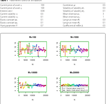
Figure 1Vulnerable call option of different values ofMandN

In the following section, we present some simulation results to examine how the parame-ters of the mixed fractional CEV model affect the valuation of the vulnerable call option. All our numerical results have been performed with the parameters in Table1.

Example1 Ifκ1=κ2= 0,σ1=σ2= 0,v2(0) = 0, andH= 0.5, then we havev1(t) = 0.05 and

v2(t) = 0. The value of the vulnerable call at current timethas the closed form

c(t,s1,s2)

=s1N2

d+(T–t,s1/K) +

v1(T–t),d–(T–t,s2/D) +ρ

v1(T–t),ρ

–Kexp–r(T–t)N2

d+(T–t,s1/K),d–(T–t,s2/D),ρ1

+(1 –α)

D s2exp

(r+ρ√v1v2)(T–t)

N2(d1,d2,ρ)

+(1 –α)s2K

D N2(d3, –d4,ρ), (5.11)

whereN2is the bivariate normal cumulative distribution function, and

d+(t,s1) =

lns1+ (r+ 0.5v1)t √

v1t

, d–(t,s2) =

lns2+ (r+ 0.5v2)t √

v2t

Figure 2Vulnerable call option of different values ofKands1

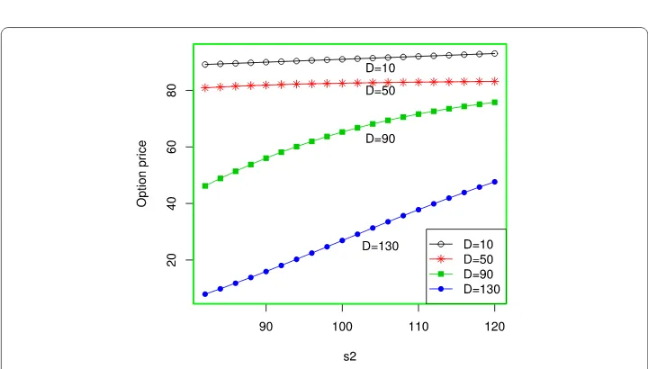
Figure 3Vulnerable call option for different values ofDands2

d1=d+(T–t,s1/K) +

v1(T–t) +ρ

v2(T–t),

d2=d–(T–t,s2/D) –ρ

v1(T–t) –

v2(T–t),

d3=d+(T–t,s1/K) +ρ

v2(T–t), d4=d–(T–t,s2/D) +

v2(T–t).

Here we compare the value of the vulnerable call using the scheme (5.7)–(5.10) with the explicit one obtained by (5.11). Figure1shows the price of the vulnerable call option with various values ofMandN. In the figure,cˆM,N(t,S1(t),S2(t)) converges toc(t,s1,s2)

as (M,N)→(∞,∞). We also show the properties of option prices in Fig.2, which shows accurate approximations for large numbersM(i.e., M= 20,000) and how the prices of vulnerable call change with respect to the asset prices1and strike priceK.

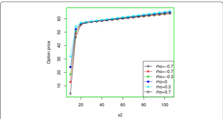
Figure 4Vulnerable call option for different values ofρ1ands2

Example2 In this example, we consider the valuation of the vulnerable call option under the mixed fractional CEV model (1.2)–(1.3). LetM= 2,000,000 andN= 20,000. Figure3

shows the valuation of the vulnerable call option for five amounts of claimsD= 10,D= 50,

D= 90, andD= 130 with differents2. In Fig.3, we observe that the option price has a

decreasing trend of theDand an increasing trend of thes2. Figure4shows the valuation

of the vulnerable call option with respect to correlationρ1ands2.

Acknowledgements

The author is sincerely grateful to the reviewer and the Associate Editor handling the paper for their valuable comments.

Funding

This work was supported by National Nature Science Foundation of China (Grant No. 71171164), Foundation of Guizhou Science and Technology Department (Grant No. 2015 2076), and Scientific research Foundation of Shaanxi Railway Institute (Grant No. KY2019-42).

Competing interests

The author declares that he has no competing interests.

Authors’ contributions

This is a single-authored paper. The author read and approved the final manuscript.

Publisher’s Note

Springer Nature remains neutral with regard to jurisdictional claims in published maps and institutional affiliations.

Received: 29 January 2019 Accepted: 17 July 2019 References

1. Lo, C.C., Nguyen, D., Skindilias, K.: A unified tree approach for options pricing under stochastic volatility models. Finance Res. Lett.20, 260–268 (2017)

2. Wang, G., Wang, X., Zhou, K.: Pricing vulnerable options with stochastic volatility. Physica A485, 91–103 (2017) 3. Jaber, E.A., Euch, O.E.: Markovian structure of the Volterra Heston model. Stat. Probab. Lett.149, 63–72 (2019) 4. Jacquier, A., Roome, P.: Large-maturity regimes of the Heston forward smile. Stoch. Process. Appl.126, 1087–1123

(2016)

5. Hull, J., White, A.: The pricing of options on assets with stochastic volatilities. J. Finance42, 281–300 (1987) 6. Xu, X., Taylor, S.: The term structure of volatility implied by foreign exchange options. J. Financ. Quant. Anal.29, 57–74

(1994)

7. Bates, D.: Post-’87 crash fears in the S&P 500 futures option market. J. Econom.94, 181–238 (2000) 8. Christoffersen, P., Jacobs, K., Ornthanalai, C., et al.: Option valuation with long-run and short-run volatility

components. J. Financ. Econ.90, 272–297 (2008)

10. Wang, G., Wang, X., Wang, Y.: Rare shock, two-factor stochastic volatility and currency option pricing. Appl. Math. Finance21, 32–50 (2014)

11. Siu, T., Yang, H., Lau, J.: Pricing currency options under two-factor Markov-modulated stochastic volatility models. Insur. Math. Econ.43, 295–302 (2008)

12. Barczy, M., Alaya, M.B., Kebaier, A., et al.: Asymptotic behavior of maximum likelihood estimators for a jump-type Heston model. J. Stat. Plan. Inference198, 139–164 (2019)

13. Kim, J., Kim, B., Moon, K., et al.: Valuation of power options under Heston’s stochastic volatility model. J. Econ. Dyn. Control36, 1796–1813 (2012)

14. Mehrdoust, F., Najafi, A.R., Fallah, S., et al.: Mixed fractional Heston model and the pricing of American options. J. Comput. Appl. Math.330, 141–154 (2018)

15. Cheridito, P.: Arbitrage in fractional Brownian motion models. Finance Stoch.7(4), 533–553 (2003)