R E S E A R C H
Open Access
On the Gabor frame set for compactly
supported continuous functions
Ole Christensen
1, Hong Oh Kim
2and Rae Young Kim
3**Correspondence: [email protected] 3Department of Mathematics,
Yeungnam University, 280 Daehak-Ro, Gyeongsan, Gyeongbuk 38541, Republic of Korea Full list of author information is available at the end of the article
Abstract
We identify a class of continuous compactly supported functions for which the known part of the Gabor frame set can be extended. At least for functions with support on an interval of length two, the curve determining the set touches the known obstructions. Easy verifiable sufficient conditions for a function to belong to the class are derived, and it is shown that the B-splinesBN,N≥2, and certain
‘continuous and truncated’ versions of several classical functions (e.g., the Gaussian and the two-sided exponential function) belong to the class. The sufficient conditions for the frame property guarantees the existence of a dual window with a prescribed size of the support.
MSC: 42C15; 42C40
Keywords: Gabor frames; frame set; B-splines
1 Introduction
Frames is a functional analytic tool to obtain representations of the elements in a Hilbert space as a (typically infinite) superposition of building blocks. Frames indeed lead to de-compositions that are similar to those obtained via orthonormal bases, but with much greater flexibility, due to the fact that the definition is significantly less restrictive. For example, in contrast to the case for a basis, the elements in a frame are not necessarily (linearly) independent, that is, frames can be redundant.
One of the main manifestations of frame theory is within Gabor analysis, where the aim is to obtain efficient representations of signals in a way that reflects the time-frequency distribution. For any a,b> , consider the translation operator Ta and the
modula-tion operatorEb, both acting on the particular Hilbert spaceL(R), given byTaf(x) =
f(x–a) andEbf(x) =eπibxf(x), respectively. Giveng∈L(R), the collection of functions {EmbTnag}m,n∈Zis called a (Gabor)frameif there exist constantsA,B> such that
Af≤
m,n∈Z
f,EmbTnag
≤Bf, ∀f ∈L(R).
If at least the upper condition is satisfied,{EmbTnag}m,n∈Zis called aBessel sequence.It is known that for every frame{EmbTnag}m,n∈Z, there exists a dual frame{EmbTnah}m,n∈Zsuch
that eachf∈L(R) has the decomposition
f =
m,n∈Z
f,EmbTnahEmbTnah. (.)
The problem of determiningg∈L(R) and parametersa,b> such that{E
mbTnag}m,n∈Zis
a frame has attracted a lot of attention over the past years. Theframe setfor a function
g∈L(R) is defined as the set
Fg:=
(a,b)∈R+| {EmbTnag}m,n∈Zis a frame forL(R).
Clearly, the ‘size’ of the set Fg reflects the flexibility of the function g in regard of
ob-taining expansions of type (.). In particular, it is known that ab≤ is necessary for
{EmbTnag}m,n∈Zto be a frame and that the number (ab)–is a measure of the redundance
of the frame; the smaller the number, the more redundant the frame. Thus, a reasonable functiongshould lead to a frame{EmbTnag}m,n∈Zfor values (ab)–that are reasonably close
to one. We remark thatFgis known to be open ifgbelongs to the Feichtinger algebra; see
[, ].
Until recently, the exact frame set was only known for very few functions: the Gaus-sian g(x) =e–x [–], the hyperbolic secant [], and the functions h(x) =e–|x|, k(x) =
e–xχ
[,∞[(x) [, ]. In [] a characterization was obtained for the class of totally positive
functions of finite type, and based on [], the frame set for functionsχ[,c], c> , was
characterized in [].
For applications of Gabor frames, it is essential that the windowgis a continuous tion with compact support. Most of the related literature deals with special types of func-tions like truncated trigonometric funcfunc-tions or various types of splines; see [–]. Vari-ous classes of functions have also been considered, for example, functions yielding a par-tition of unity [, ], functions with short support or a finite number of sign-changes [–], or functions that are bounded away from zero on a specified part of the support []. The case of B-spline generated Gabor systems has attracted special attention; see, for example, [, –]. Interesting results in the rational case are obtained in [].
To the best of our knowledge, the frame set has not been characterized for any func-tiong∈Cc(R)\ {}. We will, among others, consider a class of functions for which we
can extend the known set of parameters (a,b) yielding a Gabor frame. The class of func-tions contains the B-splinesBN,N≥, and certain ‘continuous and compactly supported
variants’ of the mentioned functionsg,hand other classical functions. Furthermore, the results guarantee the existence of dual windows with a support size given in terms of the translation parameter.
In the rest of this introduction, we will describe the relevant class of windows and their frame properties. Proofs of the frame properties are in Section , and easy verifiable con-ditions for a function to belong to the class are derived in Section .
Let us first collect some of the known results concerning frame properties for continuous compactly supported functions; (i) is classical, and we refer to [] for a proof.
Proposition . Let N > ,and assume that g:R→Cis a continuous function with suppg⊆[–N,N].Then the following holds:
(ii) []Assume that <a<N, <b≤N+a,andinfx∈[–a
,a]|g(x)|> .Then
{EmbTnag}m,n∈Zis a frame,and there is a unique dual windowh∈L(R)such that supph= [–a,a].
(iii) []Assume thatN ≤a<Nand <b<a.Ifg(x) > ,x∈]–N,N[,then {EmbTnag}m,n∈Zis a frame.
We will now introduce the window class that will be used in the current paper; it is a subset of the set of functionsgconsidered in Proposition .(iii). The definition is inspired by certain explicit estimates for B-splines given by Trebels and Steidl []; this point will be clear in Proposition .. First, fixN> and <a<N. Consider the first-order difference
af and the second-order differenceaf given by
af(x) =f(x) –f(x–a), af(x) =f(x) – f(x–a) +f(x– a).
We define the window class as the set of functions
VN,a:=
f ∈C(R)suppf =
–N ,
N
,f is real-valued and satisfies (A)-(A) ,
where
(A) f is symmetric around the origin;
(A) f is strictly increasing on[–N, ]; (A) Ifa<N
, then
af(x)≥,x∈[–N, –
N
+ a
]; ifa≥
N
, then
af(x)≥,x∈[–N
, ]∪ {–
N
+ a
}.
Note that by the symmetry condition (A) a functionf ∈VN,ais completely determined
by its behavior forx∈[–N, ]. Ifa≥N, then the point –N+a considered in (A) is not contained in [–N, ]; however, if desired, the symmetry condition allows us to formulate the condition
af(–N + a
)≥ alternatively as
f
N
– a
– f
–N –
a
≥ (.)
because the argumentx– aof the last term in the second-order difference is less than –N.
The definition of VN,a is technical, but we will derive easy verifiable conditions for a
functiongto belong to this set in Proposition . and also provide several natural examples of such functions. Our main result extends the range ofb> yielding a frame, compared with Proposition .(ii):
Theorem . For N> ,let <a<N and N+a <b≤N+a.Assume that g∈VN,a.Then
the Gabor system{EmbTnag}m,n∈Zis a frame for L(R),and there is a unique dual window
h∈L(R)such thatsupph⊆[–a
, a
].
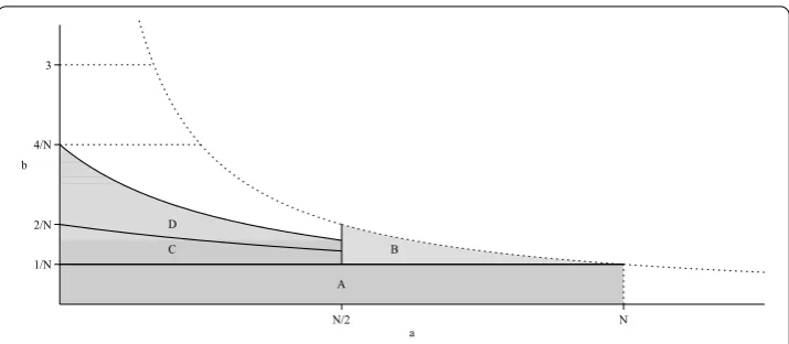
For an illustration of Proposition . and Theorem ., see Figure .
Membership of a functiong in a set VN,a for some a∈],N[ only gives information
about the frame properties of{EmbTnag}m,n∈Zfor this specific value of the translation
pa-rametera. In order to get an impression of the frame properties of{EmbTnag}m,n∈Zin a
in-Figure 1 The Gabor frame set.The figure shows the following regions:Bas in Proposition 1.1(iii), andDas in Theorem 1.2. The regionAcorresponds to the case where the frame operator is a multiplication operator, and
{EmbTnag}m,n∈Zis a frame if infx∈[0,a]n∈Z|g(x–na)|2> 0. The regionCis a part of the region determined by
Proposition 1.1(ii), corresponding to the new findings in the paper [21].
terval ofa-values, preferably for alla∈],N[. Fortunately, several natural functions have this property. The following list collects some of the results we will obtain in Section . Considering anyN∈N\ {},
• The B-splineBN of orderNbelongs to
<a<NVN,a;
• The functionfN(x) :=cosN–(πNx)χ[–N,N](x)belongs to
<a<NVN,a;
• The functionhN(x) := (e–|x|–e–
N )χ
[–N,N](x)belongs to
<a<NVN,a;
• The functiongN(x) := (e–x
–e–N)χ
[–N,N](x)belongs to
N
≤a<NVN,a.
In particular, Proposition . and Theorem . imply that forN∈N\ {}, the functions
BN,fN, andhN generate frames whenever <a<Nand <b≤N+a, andgN generates a
frame whenever N ≤a<Nand <b≤N+a.
Note that the limit curveb=N+a in Theorem . touches the known obstructions for Gabor frames. In fact, forN= , we obtain thatb→ asa→. Since it is known that the B-splineBdoes not generate a frame forb= [, ], we cannot go beyond this. We
also know that at least for some functionsg∈<a<NVN,a, parts of the region determined
by the inequalitiesb< ,a< ,ab< do not belong to the frame set. Considering, for example, the B-splineB[] shows that the point (a,b) = (,) does not belong to the
frame set. Fora=
, Theorem . guarantees the frame property forb<
, which is close
to the obstruction. These considerations indicate that the frame region in Theorem . in a quite accurate way describes the maximally possible frame set belowb= that is valid for all the functions inVN,a, at least forN= .
2 Frame properties for functionsg∈VN,a
The purpose of this section is to prove Theorem .. Since the functionsg∈VN,a are
bounded and have compact support, they generate Bessel sequences{EmbTnag}m,n∈Zfor
alla,b> . By the duality conditions [, ] two bounded functionsg,hwith compact support generate dual frames{EmbTnag}m,n∈Zand{EmbTnah}m,n∈Zfor some fixeda,b> if and only if
m∈Z
g(x–/b+ma)h(x+ma) =bδ,, a.e.x∈
–a ,
a
[image:4.595.119.477.80.236.2]
in particular, a functiong∈VN,aand a bounded real-valued functionhwith support on
[–a,a] generate dual Gabor frames{EmbTnag}m,n∈Z and{EmbTnah}m,n∈Z forL(R) for someb≤N+aif and only if, for= ,±,
m=–
g(x–/b+ma)h(x+ma) =bδ,, a.e.x∈
–a ,
a
. (.)
Giveng∈VN,a, we therefore consider the × matrix-valued functionGon [–a,a]
de-fined by
G(x) :=g(x–b+ma)
–≤,m≤=
⎛ ⎜ ⎝
g(x+b–a) g(x+b) g(x+b+a)
g(x–a) g(x) g(x+a)
g(x–b–a) g(x–b) g(x–b+a)
⎞ ⎟ ⎠.
In terms of theG(x), condition (.) simply means that
G(x)
⎛ ⎜ ⎝
h(x–a)
h(x)
h(x+a)
⎞ ⎟ ⎠=
⎛ ⎜ ⎝
b
⎞ ⎟
⎠, a.e.x∈
–a ,
a
. (.)
We will show that the matrixG(x) is invertible for allx∈[–a,a]; this will ultimately give us a bounded and compactly supported functionhsatisfying (.) and hereby prove Theorem .. The invertibility ofG(x) will be derived as a consequence of a series of lem-mas, where we first considerx∈[–a, ]. Note that the proof of the first result does not use property (A).
Lemma . For N> ,let <a<N and
N+a <b≤
N+a.Assume that g∈VN,a and let
x∈[–a, ].Then the following hold:
(a) g(x+b+a)≤g(x+b) <g(x+b–a)= ; (b) g(x–b–a)≤g(x–b) <g(x–b+a)= ;
(c) g(x) >g(x–a)andg(x)≥g(x+a)with equality only forx= –a. Proof For (a), letx∈[–a, ]. Usingb≤N+a anda<N, we have
x+
b –a≥
b–
a
≥
N+ a
–
a
> –
N
.
It follows that
x+
b –a⊆
b –
a
,
b–a
⊆
–N ,
N
. (.)
Using thatb≤N+a<a, it follows that –x–b+a≤(a–b) < ; thus,
–x–
b+a<x+
b. (.)
symmetry ofgthat
g
x+
b–a
=g
–x–
b+a
>g
x+
b
≥g
x+
b+a
;
ifx+b–a> , then we haveg(x+b–a) >g(x+b)≥g(x+b+a). Hence, (a) holds. Similarly,
(b) and (c) hold.
We now show that ifg∈VN,aanda≥N/, then condition (A) automatically holds on
a larger interval.
Lemma . For N> ,let <a<N.Assume that g∈VN,a.Thenag(x)≥for all x∈
[–N, –N +a].
Proof It suffices to show that, fora≥N
,
ag(x)≥, ∀x∈
, –N +
a
.
We first note that (A) and (A) imply that, forx∈[, –N
+ a
],
g(x)≥g
–N +
a
and g(x–a)≤g
–N –
a
. (.)
Fora≥N, we have –N–a < –N; due to the compact support ofg,f(–N–a) = ; thus using (A) again, we have
ag
–N +
a
=g
–N +
a
– g
–N –
a
=g
N
– a
– g
–N –
a
.
Together with (.), this shows that
≤ag
–N +
a
≤ag(x), ∀x∈
, –N +
a
,
as desired.
LetGij(x) denote theijth minor ofG(x), the determinant of the submatrix obtained by
removing theith row and thejth column fromG(x).
Lemma . For N> ,let <a<N and N+a <b≤N+a.Assume that g∈VN,a and let
x∈[–a
, ].Then the following hold:
(a) G(x)≥,and equality holds iffg(x+b) =g(x+b+a) = ;
(b) G(x)≥,and equality holds iffg(x–b–a) =g(x–b) = ;
Proof Sinceg≥, (a) and (b) follow from Lemma .(a), (b). For (c), we note thatag(x) =
g(x) –g(x–a) =g(–x) –g(–x+a) = –ag(–x+a) by the symmetry ofg. Now a direct
calculation shows that
G(x) –G(x) –G(x)
= –ag
x+
b
ag
x–
b+a
+ag
x+
b+a
ag
x–
b
=ag
–x–
b+a
ag
x–
b +a
–ag
–x–
b
ag
x–
b
.
Hence, it suffices to show that
ag
x–
b+a
≥ag
x–
b
, x∈
–a ,
and
ag
–x–
b +a
≥ag
–x–
b
, x∈
–a ,
or, equivalently, thatag(x–b+a)≥ andag(–x–b+a)≥, both forx∈[–a, ]. Since [–b+a, –b+a]∪[–b+a, –b+a] = [–b+a, –b+a], this means precisely that
ag(x)≥, x∈
–
b+ a
, –
b+
a
. (.)
We note that, for
N+a<b≤
N+a,
–N ≤–
b +
a
, –
b+
a
≤–
N
+ a
.
Together with Lemma ., this implies that (.) holds, as desired.
After this preparation, we can now show thatG(x) is indeed invertible forx∈[–a,a] under the assumptions in Theorem ..
Corollary . For N> ,let <a<N and N+a<b≤N+a.Assume that g∈VN,a.Then
detG(x)= for x∈[–a,a].
Proof First, considerx∈[–a, ]. By Lemma .(c) we have
detG(x) = –g(x–a)G(x) +g(x)G(x) –g(x+a)G(x)
≥–g(x–a)G(x) +g(x)
G(x) +G(x)
–g(x+a)G(x)
=g(x) –g(x–a)G(x) +
g(x) –g(x+a)G(x)
=:AN(x).
Using Lemma .(c) and Lemma .(a), (b), we have
g(x) –g(x–a)G(x)≥ and
Thus,AN(x)≥,x∈[–a, ]. IfAN(x) > for allx∈[–a, ], then the proof is completed;
thus, the rest of the proof is focused on the case whereAN(x) = for somex∈[–a, ].
In this case, Lemma .(c) shows that either
G(x) = , G(x) = (.)
or
G(x) = , x= –
a
. (.)
The case (.) actually cannot occur. Indeed, ifG(–a) = , then by Lemma .(a) we have
g(–a+b) = ; by the symmetry ofgthis would imply thatg(a–b) = , which contradicts Lemma .(b) withx= –a. Thus, we only have to deal with the case (.). IfG(x) =
G(x) = , then by Lemma .(a), (b) we have
g
x+
b
=g
x+
b+a
=g
x–
b–a
=g
x–
b
= .
Inserting this information into the entries of the matrixG(x) and applying Lemma .
yield that
detG(x) =g
x+
b–a
g(x)g
x–
b +a
> ,
as desired. This completes the proof thatG(x) > forx∈[–a, ]. Sincegis symmetric around the origin, we have
detG(–x) =det
g(–x–b+ma)
–≤,m≤=det
g(x+b–ma)
–≤,m≤
= –det
g(x– b–ma)
–≤,m≤=det
g(x– b+ma)
–≤,m≤
=detG(x).
Thus,G(x) is also invertible forx∈],a].
We are now ready to prove Theorem ..
Proof of Theorem. By Corollary . and the continuity ofg,infx∈[–a
,a]|detG(x)|> . We definehon [–a
, a
] by
⎛ ⎜ ⎝
h(x–a)
h(x)
h(x+a)
⎞ ⎟
⎠=G–(x)
⎛ ⎜ ⎝
b
⎞ ⎟ ⎠, x∈
–a ,
a
,
which is a bounded function. On R\[–a,a], puth(x) = . It follows immediately by
definition ofhthat thengandhare dual windows.
In fact, if <b≤ N+a, then the first row ofG(x) forx∈[N – b+a,a] is the zero vec-tor, and the third row ofG(x) forx∈[–a,b –a– N] is the zero vector. Hence, we have
infx∈[–a,a]detG(x) = .
The conditions forg∈VN,aare technical. We will now give an example, showing that
the conclusion about the size of the support of the dual window in Theorem . may break down ifg∈/VN,a.
Example . Let us consider the parametersN = ,a= . Consider a symmetric and continuous functiongonRwithsuppg= [–,]; assume further thatg is increasing on [–N, ] = [–, ] and that
g() = , g(–) = , g
–
= , g
–
= .
Thenag(–) =g(–) – g(–) +g(–) = – < . Hence,gdoes not satisfy (A) atx= –, that is,g∈/VN,a.
We will show that, forb=N+a=, there does not exist a bounded real-valued function
h∈L(R) withsupph⊆[–a
, a
] such that the duality conditions (.) hold. In order to
obtain a contradiction, let us assume that such a dual window indeed exists. Letx= .
Then
x–a= –x–a= –, x–
b+a= –x–
b+a= –
,
x–
b= –x–
b= –
, x–
b–a= –x–
b–a= –
,
and, consequently,
G(x) =
⎛ ⎜ ⎝
g(x+b–a) g(x+b) g(x+b+a)
g(x–a) g(x) g(x+a)
g(x–b–a) g(x–b) g(x–b+a)
⎞ ⎟ ⎠=
⎛ ⎜ ⎝
⎞ ⎟ ⎠.
By the continuity ofgthere exist continuous functionsij(x), ≤i,j≤, such that
G(x) =
⎛ ⎜ ⎝
+(x) +(x) (x)
+(x) +(x) +(x)
(x) +(x) +(x)
⎞ ⎟ ⎠
and
ij(x)→ asx→x.
Then (.) implies that
⎛ ⎜ ⎝
+(x) +(x) (x)
+(x) +(x) +(x)
(x) +(x) +(x)
⎞ ⎟ ⎠
⎛ ⎜ ⎝
h(x–a)
h(x)
h(x+a)
⎞ ⎟ ⎠=
⎛ ⎜ ⎝
b
for a.e.x∈[–a,a]. By elementary row operations this leads to
⎛ ⎜ ⎝
+(x) +(x) (x)
η(x) η(x) η(x)
(x) +(x) +(x)
⎞ ⎟ ⎠
⎛ ⎜ ⎝
h(x–a)
h(x)
h(x+a)
⎞ ⎟ ⎠=
⎛ ⎜ ⎝
b
⎞ ⎟
⎠, a.e.x∈
–a ,
a
,
whereηi(x) :=i(x) – i(x) – i(x) for ≤i≤. Sincehis a bounded function, ignoring
a possible set of measure zero, this implies that
b=η(x)h(x–a) +η(x)h(x) +η(x)h(x+a)→
asx→x. This is a contradiction.
On the other hand, the condition g∈VN,a is not necessary for{EmbTnag}m,n∈Z to be
a frame in the considered region. For example, let N= ,a=,b= and takeg(x) :=
(e–x –e–)χ
[–,](x). Then elementary calculations show that (A) does not hold for
x∈[–, –]⊂[–N, –N +a]. But sincedetG(x) > forx∈[–a,a], we can prove that
{EmbTnag}m,n∈Zis a frame by following the steps in the proof of Theorem ..
3 The setVN,a
In this section, we give easily verifiable sufficient conditions for a functiong to belong toVN,a. Recall that a continuous functionf :R→Cwithsuppf = [–N,N] is piecewise
continuously differentiable if there exist finitely manyx= –N <x<· · ·<xn=N such
that
() f is continuously differentiable on]–xi–,xi[for everyi∈ {, . . . ,n};
() the one-sided limitslimx→x+
i–f
(x)andlimx→x– i f
(x)exist for everyi∈ {, . . . ,n}.
Note that ifgis a continuous and piecewise continuously differentiable function, then the fundamental theorem of calculus yields that
ag(x) = x
x–a
g(t)dt for allx∈R,a> . (.)
In order to avoid a tedious presentation, we will forego to mention the points where a piecewise continuously differentiable function is not differentiable, for example, in condi-tions (c) and (d) in the following Proposition .. The result is inspired by explicit calcula-tions for B-splines in Trebels and Steidl [], Lemma .
Proposition . Let N> and assume that a continuous and piecewise continuously dif-ferentiable function g:R→Rwithsuppg= [–N,N]satisfies the following conditions:
(a) gis symmetric around the origin; (b) gis strictly increasing on[–N, ];
(c) gis increasing on]–N
, –
N
];
(d) g(–x–N)≤g(x)forx∈[–N, [. Then g∈ ∩<a<NVN,a.
consideration then extends the result to the case of piecewise differentiable functions. Let us first considerx≤–N. Then, by the mean value theorem,
ag(x) =a
g(x) –g(x–a)
a –
g(x–a) –g(x– a)
a
=ag(ξ) –g(η)
for someη∈[x– a,x–a],ξ∈[x–a,x]. Sincegis increasing up tox= –N, this proves thatag(x)≥ wheneverx≤–N.
We now considerx∈[–N,min(–N+a, )]. Then
x–a≤min
–N –
a
, –a
≤–N
and
ag(x) =
–N
x–a
g(t) –g(t–a)dt+
x
–N
g(t) –g(t–a)dt
≥ –N
x–a
g(t) –g(t–a)dt+
x
–N
g
–t–N
–g(t–a)
dt =g –N –g –N –a
–g(x–a) +g(x– a)
–g
–x–N
–g(x–a) +g
N – N +g –N –a
=g –N
–g(x–a) –
g
–a–N
–g(x– a)
(.) +g –N
–g(x–a) –
g
–x–N
–g
–a–N
. (.)
We now consider the terms (.) and (.) separately. For (.), by the mean value theorem,
g
–N
–g(x–a) –
g
–a–N
–g(x– a)
=
–N –x+a
g(–N
) –g(x–a)
–N –x+a –
g(–a–N
) –g(x– a)
–N –x+a
=
–N –x+a
g(ξ) –g(η)
for someη∈[x– a, –a–N
],ξ∈[x–a, –
N
]. Since –a–
N
≤x–a, we haveη≤ξ≤–
N
;
thus, by assumption (c),g(η)≤g(ξ). Recalling thatx≤–N +a< –N+a, we have–N –
x+a> ; thus, we conclude that the term in (.) indeed is nonnegative.
For (.), we consider two cases. Ifx–a≥–x–N, then exactly the same argument as for (.) works. Ifx–a< –x–N, then we perform the same argument after a rearrangement of the terms. Indeed,
g
–N
–g(x–a) –
g
–x–N
–g
–a–N =g –N –g
–x–N
–
g(x–a) –g
–a–N
=
x+N
g(–N) –g(–x–N)
x+N –
g(x–a) –g(–a–N)
x+N
=
x+N
g(ξ) –g(η)
for someη∈[–a–N,x–a],ξ∈[–x–N, –N]. As before, this implies that (.) is nonneg-ative.
We now considerx= –N+a; according to (.), we must prove that
g N – a
– g
–N – a ≥. (.)
First, ifa>N (i.e., –N+a>N), then we have
g N – a
– g
–N – a
=N–a
g(N –a) –g(–N –a)
N–a
–g(–
N
–
a
) –g( –N
+
a
)
N–a
=N–a
g(ξ) –g(η)
for someξ∈[–N –a,N –a],η∈[–N +a, –N–a]; thus, (.) holds by assumption (c). Now assume thatN <a≤N; then –N +a≤N, and
–N ≤ N – a ≤, – N – a
< –
N
+
a
< .
Thus, g N – a
– g
–N – a ≥g –N –g –N – a – g –N – a –g –N – a ;
this can again be expressed in terms of the differenceg(ξ) –g(η) withξ∈[–N
–
a
, –
N
],
η∈[–N –a, –N–a] and is hence positive.
Finally, we assume that N ≤a≤N. Then –N +a ≤N; since –N –a< –a, assump-tion (b) implies that
g N – a –g –N – a ≥g N – a –g –a ≥ N –a
–a
g(t)dt=: (∗).
Since –N ≤–a <N –a ≤, (d) implies that
(∗)≥
N –a
–a g
–t–N
dt=
–N+a –N+a
Since –N +a ≤–N andgis increasing on ]–∞, –N], shifting the integration interval by –N +a≥ to the left yields that
(∗∗)≥
–N–a –N
g(t)dt=g
–N –
a
;
thus, (.) holds, as desired.
Proposition . immediately leads to the following simple criterion for a function to belong to<a<NVN,a.
Corollary . Let N> and assume that a continuous and piecewise continuously differ-entiable function g:R→Rwithsuppg= [–N,N]satisfies the following conditions:
(a) gis symmetric around the origin; (b) gis positive and increasing on]–N, [. Then g∈<a<NVN,a.
We will now describe several functions belonging toVN,a, either for allafrom ],N[ or
from a subinterval hereof.
Example . Consider the B-splinesBN,N∈N, defined recursively by
B=χ[–/,/], BN+=BN∗B.
In [], Lemma , it is proved that, forN∈N\ {},
(i) BN is increasing on]–N, –N +]; (ii) BN(–x–N)≤BN(x)forx∈[–N, [.
Thus, Proposition . implies thatBN∈
<a<NVN,aforN∈N\ {}.
Example . LetN∈N\ {}and define
fN(x) :=cosN–
πx N
χ[–N
,N](x).
Direct calculations show that, forx∈]–N, –N],
fN(x) = (N– )π
N cos
N–
πx
N
(N– )sin
πx
N
–cos
πx
N
≥
and, forx∈[–N, [,
fN(x) –fN
–x–N
=(N– )π
N sin
πx N
sinN–
πx
N
–cosN–
πx
N
≥.
By Proposition .,fN ∈
<a<NVN,a.
Example . LetN> and define
hN(x) :=
e–|x|–e–Nχ
[–N,N](x).
ThenhN∈
<a<NVN,aby Corollary ..
Example . LetN> and define
kN(x) :=
+|x|–
+N
χ[–N
,N](x). ThenkN∈
<a<NVN,aby Corollary ..
In the following examples simple sufficient conditions in Proposition . and Corol-lary . are not satisfied. We will use the definition directly to show that the considered functions belong toVN,afor certain ranges of the parametera.
Example . LetN> and consider
pN(x) :=
+x –
+ (N)
χ[–N
,N](x). We will show that
(a) pN∈N
≤a<NVN,a;
(b) pN∈
N
≤a<N VN,aifN≥
≈.· · ·.
It is clear that (A) and (A) hold, so for the considered values ofa, we now check (A). In fact, we will prove more, namely that
apN(x)≥, x∈
–N , –
N
+ a
. (.)
Considering anya∈[N
,N[, we have
–N < –
N
+ a
<
N
, a–
N
< –
N
+ a
<a+
N
, –
N
+ a
< a–
N
;
so the fact thatpN > on ]–N,N[,pN(·–a) > on ]a–N,a+N[, andpN(·– a) > on
]a–N, a+N[ immediately shows that
() pN(x)= ,x∈] –N, –N +a];
() pN(x–a) = ,x∈[–N,a–N];pN(x–a)= ,x∈]a–N, –N +a];
() pN(x– a) = ,x∈[–N, –N +a].
Thus,
apN(x) =
pN(x), x∈[–N, –N +a],
pN(x) – pN(x–a), x∈]–N +a, –N+a].
SincepN(x)≥,x∈[–N, –N +a], it now suffices to prove that
pN(x) – pN(x–a)≥, x∈
–N +a, –
N
+ a
Letx∈]–N +a, –N +a]. We see that
pN(x) – pN(x–a) =pN(x) –pN(x–a) –pN(x–a)
=
+x –
+ (x–a)–
+ (x–a) –
+ (N)
= (x–a)
–x
( +x)( + (x–a))–
(N
)
– (x–a)
( + (x–a))( + (N
))
. (.)
In order to prove (a), we now assume thatN ≤a<N. Sincex≤(N)and (x–a)–x≥
, we have
pN(x) – pN(x–a)≥
(x–a)–x
( + (N))( + (x–a))–
(N)– (x–a) ( + (x–a))( + (N
))
= h(x)
( + (N))( + (x–a)),
where
h(x) := (x–a)–x–N
= (x– a)
– a–N
.
Note that the quadratic functionhis symmetric aroundx= a. Since –N +a < aand
N
≤a<N, we have
h(x)≥h
–N +
a
=
(N–a)(a– N)≥. (.)
Thus,
pN(x) – pN(x–a)≥.
Therefore, (.) holds, that is, the proof of (a) is completed. In order to prove (b), assume now thatN≥
and
N
≤a< N
. Since (x–a) –x=
a(a–x) and (N)– (x–a)= (N –x+a)(N +x–a), (.) implies that
pN(x) – pN(x–a) =
+ (x–a)
a(a–x) +x –
(N –x+a)(N +x–a) + (N)
.
Using –N +a<x≤–N +a, it follows thatN –x+a<NandN +x–a≤N –a≤–x+a; thus,
pN(x) – pN(x–a)≥
+ (x–a)
a(a
–x)
+x –
N(a
–x)
+ (N)
=
a
–x
+ (x–a)
q(x) ( +x)( + (N
))
whereq(x) := a( + (N)) –N( +x). Since N
≤a< N
and –
N
+a<x≤–
N
+ a
, we
have –N
<x≤
N
; sox <N
. Thus,
q(x)≥N
+
N
–N
+N
=N
– +
N
≥.
Thus,pN(x) – pN(x–a)≥. Therefore, (.) holds, as desired.
Example . LetN> and consider
gN(x) :=
e–x–e–N χ
[–N,N](x). We will show thatgN ∈
N
≤a<NVN,a. As in Example . (see (.)), it suffices to check that
gN(x) – gN(x–a)≥, x∈
–N +a, –
N
+ a
.
Letx∈]–N +a, –N +a], anda∈[N,N[. We see that
gN(x) – gN(x–a) =gN(x) –gN(x–a) –gN(x–a)
=e–x–e–(x–a)–e–(x–a)–e–N
=e–(x–a)e(x–a)–x– –e–N eN
–(x–a)– .
Since –(x–a)≥–N
and (x–a)–x≥, we have
gN(x) – gN(x–a)≥e–
N
e(x–a)–x– –e–N eN
–(x–a)– =e–N
e(x–a)–x–eN –(x–a) =e–(x–a)eh(x)– ,
whereh(x) := (x–a)–x– (N
). From (.) we haveh(x)≥. Thus,
gN(x) – gN(x–a)≥,
as desired.
Competing interests
The authors declare that they have no competing interests.
Authors’ contributions
All authors contributed equally to this work. All authors read and approved the final manuscript.
Author details
1Department of Applied Mathematics and Computer Science, Technical University of Denmark, Building 303, Lyngby,
2800, Denmark.2Division of General Studies, UNIST, 50 UNIST-gil, Ulsan, 44919, Republic of Korea.3Department of
Acknowledgements
The authors would like to thank the reviewers for many useful suggestions, which clearly improved the presentation. In particular, one reviewer suggested to formulate condition (A3) for membership ofVN,ain terms of second-order differences, which is much more transparent than our original condition. He also suggested the approach in the current proof of Proposition 3.1, which is shorter than our original one. This research was supported by Basic Science Research Program through the National Research Foundation of Korea (NRF) funded by the Ministry of Education
(2013R1A1A2A10011922).
Received: 25 November 2015 Accepted: 16 February 2016
References
1. Feichtinger, HG, Kaiblinger, N: Varying the time-frequency lattice of Gabor frames. Trans. Am. Math. Soc.356, 2001-2023 (2004)
2. Ascensi, G, Feichtinger, HG, Kaiblinger, N: Dilation of the Weyl symbol and the Balian-Low theorem. Trans. Am. Math. Soc.366, 3865-3880 (2014)
3. Lyubarskii, Y: Frames in the Bargmann space of entire functions. Adv. Sov. Math.11, 167-180 (1992)
4. Seip, K: Density theorems for sampling and interpolation in the Bargmann-Fock space I. J. Reine Angew. Math.429, 91-106 (1992)
5. Seip, K, Wallsten, R: Density theorems for sampling and interpolation in the Bargmann-Fock space II. J. Reine Angew. Math.429, 107-113 (1992)
6. Janssen, AJEM, Strohmer, T: Hyperbolic secants yield Gabor frames. Appl. Comput. Harmon. Anal.12, 259-267 (2002) 7. Janssen, AJEM: Some Weyl-Heisenberg frame bound calculations. Indag. Math.7, 165-183 (1996)
8. Janssen, AJEM: On generating tight Gabor frames at critical density. J. Fourier Anal. Appl.9, 175-214 (2003) 9. Gröchenig, K, Stöckler, J: Gabor frames and totally positive functions. Duke Math. J.162, 1003-1031 (2013) 10. Janssen, AJEM: Zak transforms with few zeros and the tie. In: Feichtinger, HG, Strohmer, T (eds.) Advances in Gabor
Analysis. Appl. Numer. Harmon. Anal., pp. 31-70. Birkhäuser, Boston (2003)
11. Dai, XR, Sun, Q: Theabc-problem for Gabor systems. Mem. Am. Math. Soc. (to appear)
12. Del Prete, V: Estimates, decay properties, and computation of the dual function for Gabor frames. J. Fourier Anal. Appl.
5, 545-562 (1999)
13. Laugesen, RS: Gabor dual spline windows. Appl. Comput. Harmon. Anal.27, 180-194 (2009)
14. Kloos, T, Stöckler, J: Zak transforms and Gabor frames of totally positive functions and exponential B-splines. J. Approx. Theory184, 209-237 (2014)
15. Kim, I: Gabor frames with trigonometric spline dual windows. Asian-Eur. J. Math.8(4), 1550072 (2015) 16. Gröchenig, K, Janssen, AJEM, Kaiblinger, N, Pfander, G: Note on B-splines, wavelet scaling functions, and Gabor
frames. IEEE Trans. Inf. Theory49, 3318-3320 (2003)
17. Christensen, O, Kim, HO, Kim, RY: On entire functions restricted to intervals, partition of unities, and dual Gabor frames. Appl. Comput. Harmon. Anal.38, 72-86 (2015)
18. Christensen, O, Kim, HO, Kim, RY: Gabor windows supported on [–1, 1] and compactly supported dual windows. Appl. Comput. Harmon. Anal.28, 89-103 (2010)
19. Christensen, O, Kim, HO, Kim, RY: Gabor windows supported on [–1, 1] and dual windows with small support. Adv. Comput. Math.36, 525-545 (2012)
20. Christensen, O, Kim, HO, Kim, RY: On Gabor frames generated by sign-changing windows and B-splines. Appl. Comput. Harmon. Anal.39, 534-544 (2015)
21. Lemvig, J, Nielsen, H: Counterexamples to the B-spline conjecture for Gabor frames. J. Fourier Anal. Appl. (to appear) 22. Prete, VD: Estimates, decay properties, and computation of the dual function for Gabor frames. J. Fourier Anal. Appl.5,
545-561 (1999)
23. Gröchenig, K: Partitions of unity and new obstructions for Gabor frames. Preprint
24. Lyubarskii, Y, Nes, PG: Gabor frames with rational density. Appl. Comput. Harmon. Anal.34, 488-494 (2013) 25. Christensen, O: An Introduction to Frames and Riesz Bases, 2nd expanded edn. Birkhäuser, Boston (2016) 26. Trebels, B, Steidl, G: Riesz bounds of Wilson bases generated by B-splines. J. Fourier Anal. Appl.6, 171-184 (2000) 27. Ron, A, Shen, Z: Weyl-Heisenberg systems and Riesz bases inL2(Rd). Duke Math. J.89, 237-282 (1997) 28. Janssen, AJEM: The duality condition for Weyl-Heisenberg frames. In: Feichtinger, HG, Strohmer, T (eds.) Gabor