2018-01-0193 Published 03 Apr 2018
© 2018 SAE International; Argonne National Laboratory.
Numerical Methodology for Optimization
of Compression-Ignited Engines Considering
Combustion Noise Control
Alberto Broatch, Ricardo Novella, and Josep Gomez-Soriano Universitat Politecnica de Valencia
Pinaki Pal and Sibendu Som Argonne National Laboratory
Citation: Broatch, A., Novella, R., Gomez-Soriano, J., Pal, P. et al., “Numerical Methodology for Optimization of Compression-Ignited Engines Considering Combustion Noise Control,” SAE Technical Paper 2018-01-0193, 2018, doi:10.4271/2018-01-0193.
Abstract
I
t is challenging to develop highly efficient and cleanengines while meeting user expectations in terms of performance, comfort and drivability. One of the critical aspects in this regard is combustion noise control. Combustion noise accounts for about 40 percent of the overall engine noise in typical turbocharged diesel engines. The experimental investigation of noise generation is difficult due to its inherent complexity and measurement limitations. Therefore, it is important to develop efficient numerical strat-egies in order to gain a better understanding of the combus-tion noise mechanisms. In this work, a novel methodology was developed, combining computational fluid dynamics (CFD) modeling and genetic algorithm (GA) technique to optimize the combustion system hardware design of a high-speed direct injection (HSDI) diesel engine, with respect to various emissions and performance targets including combustion noise. The CFD model was specifically set up to reproduce the unsteady pressure field inside the combustion chamber, thereby allowing an accurate prediction of the acoustic response of the combustion phenomena. The model was validated by simulating several steady operating condi-tions and comparing the numerical results against experi-mental data, in both temporal and frequency domains. Thereafter, a GA optimization was performed with the goal
of minimizing indicated specific fuel consumption (ISFC) and combustion noise, while restricting pollutant (soot and
NOx) emissions to their respective baseline values. Eight
design variables were selected pertaining to piston bowl geometry, nozzle inclusion angle, number of injector nozzle holes and in-cylinder swirl. An objective merit function based on the emissions, ISFC and combustion noise, was constructed to quantify the strength of the engine designs, and was determined using the CFD model as the function evaluator. The in-cylinder noise level was characterized by the total resonance energy of local pressure oscillations. The optimum engine configuration thus obtained, showed a significant improvement in terms of efficiency and combus-tion noise compared to the baseline system, along with both
soot and NOx emissions within their respective constraints.
This optimum configuration included a deeper and tighter bowl geometry with higher swirl and larger number of nozzle holes. Subsequently, a more detailed acoustics analysis based on proper orthogonal decomposition (POD) technique was carried out to further explore the combustion noise benefits achieved by the GA optimum. This computational study is a first of its kind (to the best of the authors’ knowledge), which demonstrates a comprehensive framework to incor-porate combustion noise into a numerical optimization strategy for engine design.
Introduction
T
he degradation of air quality due to exhaust emissionsfrom the transport vehicles has increased concerns about the pollutant emission sources over the last few decades. While the number of respiratory diseases has signifi-cantly grown in urban environments [1], the weather has also experienced noticeable changes due to global warming [2]. This situation has forced engine manufacturers to face ever-increasing exhaust emissions regulations while adhering to strict consumer demands of high fuel economy, thermal efficiency and drivability.
As a consequence of this struggle, a variety of new combustion modes [3, 4, 5] have been developed. Most of them
operate in highly premixed conditions to avoid particulate matter (PM) precursors while the generation of nitrous oxides
(NOx) is controlled via large amounts of exhaust gas
recircula-tion (EGR). A considerable number of investigarecircula-tions [6, 7] have confirmed the suitability of these combustion concepts
to achieve really low emissions of both NOx and soot
particu-lates, while maintaining or even improving the engine perfor-mance. However, high pressure rates associated with these particular modes of combustion exacerbate the NVH (Noise, Vibration and Harshness) issues and thus compromise the user’s comfort and the quality of life in populated areas [8].
phenomena to the overall noise emissions may be completely different depending on the application. For instance, in compression ignition (CI) engines operating with conven-tional diesel combustion (CDC), the pressure instabilities generated during the premixed combustion largely dominate the acoustic source, rendering the pressure oscillations induced by turbulence-combustion interaction [10, 11] secondary. Therefore, a better fundamental understanding of noise is essential for assessing the connection between combustion and its corresponding acoustics.
In addition to the pressure instability induced by combus-tion itself, the generated pressure waves resonate inside the chamber [12], interacting with the chamber walls, thereby acting as an extra acoustic source. This complex phenomenon, commonly known as combustion chamber resonance, has a significant impact on the radiated engine noise because the characteristic excitation frequency span is in the highly sensi-tive human perception range [13, 14] and its effects become especially evident during low-to-medium load operation and at transient conditions [15].
Once the acoustic excitation occurs, acoustic perturba-tions are transferred through the engine block into the vehicle and the environment. NVH analysis has demonstrated the complexity of the propagation patterns of acoustic energy [16]. Moreover, it allowed to establish a relation among acoustic response of the engine, block design and acoustic insulation [17].
Two different strategies are traditionally used to reduce noise emissions and modify the acoustic signature of the engine. The first, known as passive solution, is related to the modification of the acoustic response of the source by combining a proper engine block design and encapsulation. The second strategy, known as active solution, entails opti-mizing the hardware design and operation settings to act directly on the combustion noise source.
Passive solutions have been thoroughly explored in the past due to their inherent simplicity. Since the basis of these strategies lies in attenuating the frequency contents which have an untoward effect on NVH, the unsteady nature of the acoustic response and its highly non-linear behavior compli-cate the understanding of the radiation paths and the involved mechanisms. Nevertheless, research efforts have been made to assess the acoustic radiation through simple models, estab-lishing a relation between the combustion noise source and the end user. Anderton [18] proposed a linear behavior between the source and the observer for the engine block attenuation curve. Even though this simplification did not allow for an accurate prediction of the radiated noise level, it was useful to perform comparative analyses, and several combustion noise metrics were defined following this method. More recently, cause-effect relationships between typical combustion related parameters and free-field noise measure-ments were found [19], thereby connecting the noise source to both the objective and subjective effects of engine radiated noise [13, 14].
In contrast to passive solutions, the major difficulties in the active strategies lie in the understanding of the complex phenomena involved in noise generation and their direct effects on the in-cylinder pressure field. This demands multiple
measurement points across the combustion chamber [20] for the recreation of the unsteady pressure field and subsequent analysis, which in turn requires complex and expensive engine modifications. For this reason, most studies have resorted to numerical simulations in order to assess the noise source [21] instead. In particular, the use of computational fluid dynamics (CFD) is nowadays widely established in the automotive industry. Moreover, recent studies have demonstrated that CFD is a useful tool to recreate, visualize and study the combustion noise source [22, 23]. Despite the attractive benefits of this method, the simulation of an internal combus-tion engine is challenging due to complex geometry, spatially and temporally varying conditions and complicated combus-tion chemistry. Therefore, addicombus-tional efforts must be focused on not only developing more robust codes, but also on the validation procedure to ensure a correct estimation of the involved physical phenomena [24].
Once the simulations have been validated, any number of parameters can be modified and readily tested. This encour-aged development of additional techniques for the identifica-tion of optimizaidentifica-tion pathways with respect to combusidentifica-tion chamber design [25] or engine operating conditions [26, 27]. The interest in optimization methods based on genetic algo-rithm (GA) has increased in the automotive industry over the last few years due to the wide range of solutions they offer in combination with CFD. Several studies [28, 29] have applied this technique to diverse engine applications in which the number of optimized parameters is relatively high. For instance, Senecal and Reitz [30] optimized the combustion chamber design of a CI diesel engine with six design param-eters considering emissions and performance. Sun and Wang [31] combined GA and artificial neural network for optimizing the intake port design of a spark-ignited (SI) engine with four control parameters. However, till date, combustion noise control has not been employed as a criterion in engine design optimization studies.
In the present work, a novel numerical methodology was implemented for optimizing the combustion system in a high-speed direct injection (HSDI) diesel engine. Besides
the performance and emissions (NOx and soot), engine
noise was also included as an objective parameter. In this regard, specific considerations were made pertaining to the CFD model parameters that could affect the estimation of the in-cylinder pressure field, and subsequently, the noise emissions. Although one of the objectives of this paper was to contribute to the understanding of the relationship between noise emissions and chamber geometry in CDC, the final goal was to develop a general technique which could also be applied to new combustion modes such as Homogenous Charge Compression Ignition (HCCI) or Partially Premixed Combustion (PPC) in different engine configurations.
© 2018 SAE International; Argonne National Laboratory.
Engine Specifications and
Experimental Facility
The engine configuration is the same as that used in previous investigations by the authors [13, 14]. The tests were carried out in a light-duty HSDI diesel engine for automotive appli-cations directly coupled to an asynchronous dynamometer. It was a 1.6 L, four-cylinder, turbocharged engine equipped with a common rail injection system. The main specifica-tions of the engine and the fuel injector are summarized in Table 1.
The test bench was installed inside an anechoic chamber which guaranteed free-field conditions for frequencies above 100 Hz. In addition, the dynamometer was physically and acoustically isolated with sound damping panels to prevent possible disturbances in the noise measurements. Moreover, the rate of heat release and other relevant combustion param-eters were estimated by applying some simplifications to the energy equation [32].
Methodology
In this section, the numerical methodology and mathematical approaches outlined in the introduction are described in detail.
Numerical Model Setup
A numerical model of the engine was developed using the commercial CFD code CONVERGE v2.2 [33]. The simula-tions were performed between two consecutive exhaust valve openings (EVO), encompassing a complete engine cycle. The numerical solution of the 3D domain was obtained by using the finite volume method. A second-order central difference scheme was used for spatial discretization and a first-order implicit scheme was employed for temporal discretization.
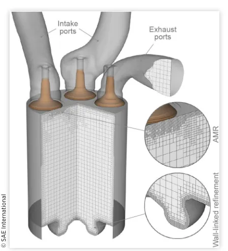
The numerical domain, as shown in Figure 1, included the complete single cylinder geometry and the intake/exhaust ports for performing full cycle simulations. The mesh discreti-zation was done using the cut-cell Cartesian method available in the code. The base mesh size was 3 mm throughout the domain. Three levels of fixed embedding (0.375 mm of cell size)
were added to the walls of the combustion chamber, ports and region near the fuel injector, to improve boundary layer prediction and the accuracy of spray atomization, droplet breakup/coalescence, etc. Mesh size in the chamber was reduced with two levels of embedding (0.75 mm of cell size) after the start of combustion, for an improved recreation of the interaction and reflection of the pressure waves. The code also employed adaptive mesh refinement (AMR) to increase grid resolution (up to 0.378 mm minimum cell size) based on the velocity and temperature subgrid scales of 1 m/s and 2.5 K, respectively. As a result, the total number of cells varied between 1.5 million at Bottom Dead Center (BDC) and 0.5 million at Top Dead Center (TDC). This mesh configura-tion was selected after a grid independence study, offering a grid-independent solution for the pertinent acoustic and combustion parameters.
The maximum sonic Courant number, based on the speed of sound, was fixed to unity during combustion to capture local fluctuations of the in-cylinder pressure field. Several monitor points were distributed across the combustion chamber in order to analyze the location of the standing waves. Moreover, the computed pressure was recorded at a sampling frequency of 50 kHz so as to provide an aliasing-free bandwidth sufficient to cover the human hearing range [34].
In-cylinder turbulence was modeled using the Reynolds-Averaged Navier Stokes (RANS) based re-normalized group
(RNG) k-ε model [35] coupled with the wall heat transfer
model developed by Angelberger et al. [36]. The Redlich-Kwong equation [37] was selected as the equation of state for calculating the compressible flow properties. Pressure-velocity coupling was achieved by using a modified Pressure Implicit with Splitting of Operators (PISO) method [38].
[image:3.612.324.548.105.352.2]Fuel injection was described by the standard Discrete Droplet Model (DDM) [39] and Kelvin Helmholtz
TABLE 1 Engine specifications and injector features.
Engine type DI diesel engine
Number of cylinders [-] 4 Displacement [cm3] 1600
Bore/Stroke [mm] 75.0/88.3 Connecting rod [mm] 13.7 Compression ratio [-] 18:1 Injector nozzle holes [-] 6 Nozzle diameter [μm] 124 Nozzle inclusion angle [deg] 150
©
S
A
E I
nt
er
na
ti
onal
FIGURE 1 A schematic of the computational domain at intake valve closing (IVO), including the intake and exhaust pipes/valves, cylinder walls and combustion chamber.
©
S
A
E I
nt
er
na
ti
(KH)-Rayleigh Taylor (RT) breakup model was employed to model spray atomization [40]. Droplet collision and coales-cence were modeled by O’Rourke’s model [41]. Moreover, the Frossling correlation [42] was used to model fuel evaporation. The drag coefficient of the droplets was calculated by the dynamic drag model of Liu et al. [43]. A reduced chemical kinetic mechanism for primary reference fuels (PRF) consisting of 42 species and 168 reactions based on Brakora et al. [44] was used in this work to account for fuel chemistry and n-heptane was used as the diesel surrogate. Regarding emissions, soot formation and oxidation were determined by
the empirical Hiroyasu soot model [45] whereas NOx
forma-tion was modeled by the extended Zel’dovich mechanism [46]. For combustion modeling, the SAGE detailed chemistry solver [47] was employed along with a multi-zone (MZ) approach, with bins of 5 K in temperature and 0.05 in equivalence ratio [48]. Although it does not utilize an explicit turbulent combustion closure [49, 50], the SAGE-MZ model has been demonstrated to perform well for simulating spray combustion in the context of RANS in previous studies [51, 52].
Cylinder wall temperatures were assumed to be constant and estimated using a lumped heat transfer model [53]. The inflow/outflow boundaries placed at the end of the intake and exhaust ports were prescribed the cycle-averaged values of the corresponding measured pressures and temperatures.
Finally, the runtime for a full cycle simulation was around 130 hours on 32 processors.
Model Validation
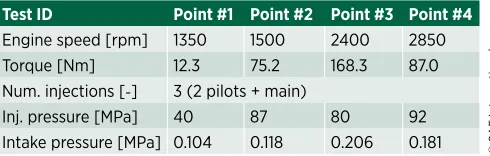
Four different steady operating conditions, summarized in Table 2, were selected to validate the numerical model. These conditions were sufficiently representative of all noise issues present in the whole operating range and the contribution of each frequency band (low, medium and high frequency) to the overall engine noise was completely different among these operation points.
Traditional in-cylinder pressure measurements through a single transducer do not provide enough information for evaluating the effects of the resonance due to local fluctuations of the pressure field. Broatch et al. [22] proposed a method-ology based on CFD simulations to overcome this limitation without complex and expensive engine modifications. They compared the simulated and measured pressure profiles at the same location of the pressure transducer and checked the consistency between numerical results and measurements in both the time and frequency domains. Then, the solution was
considered to be suitable for extrapolation to the entire domain. They also defined an elaborate procedure for choosing a representative cycle of a specific operation point. This method was specifically developed for preserving the high frequency content of the pressure signal after cycle averaging. The resulting cycle would, therefore be the most representative of the noise generated during the specific engine test.
Figure 2 shows the comparison between simulations and experiments at the four conditions considered for validation. On the left side, pressure traces registered at the transducer location in experiments and simulations are plotted along with the corresponding rates of heat release (RoHR). In general, a good agreement is obtained with experiments for all the four operating points. Zoomed views also show that the resonant oscillation process is consistently reproduced by the simulations. On the other hand, the pressure spectral density or sound pressure level (SPL) of all operation points is displayed on the right side. Numerical results overlap with measurements in almost the whole frequency range and for all the operating conditions, with only a slight disagreement observed for the medium frequencies in Points #2 and #4.
The suitability of the model for predicting noise emissions and performance levels was also assessed. The Overall Noise (ON), further explained in Appendix A, and ISFC were selected for validation. Figure 3 shows that both ON and ISFC predictions are quite reasonable, since errors between the simulations and experiments are below 1% and 10%, respec-tively. Thus, although there was a slight disagreement in the medium frequency range of the spectrum of some of the oper-ating points, the model ensures an accurate prediction of the external engine acoustic field and fuel consumption for all the operating conditions considered.
It is noted that NOx and soot emissions predicted by the
CFD model could not be compared with direct measurements as it was not possible to measure these pollutant emissions inside the anechoic chamber. Nevertheless, based on the authors’ experience, Hiroyasu soot model [45] and Zel’dovich mechanism [46] are expected to provide good estimations of
soot and NOx emissions, respectively. The authors have
employed them in various engine studies before and both emissions were reasonably well predicted when compared to exhaust analyzer measurements. Examples of such validation
can be found in Refs. [22, 52]. Therefore, the CFD soot/NOx
predictions are considered to be sufficiently representative of the real emission levels in this study.
Simplified Approach
Despite good agreement between simulations and experi-ments shown above, the CFD simulations were highly time consuming. This compromises their suitability for use with optimization techniques, such as genetic algorithms, that automatically refine the solution until an optimum is found after a large number of calculations.
Several modifications to the original model setup were, therefore, made in order to minimize the calculation time while ensuring high accuracy.
[image:4.612.56.301.672.750.2]First, the base mesh size was increased to 5 mm. All fixed embedding regions were maintained at the same levels of
TABLE 2 Main engine settings of the operation points considered for model validation.
Test ID Point #1 Point #2 Point #3 Point #4
Engine speed [rpm] 1350 1500 2400 2850
Torque [Nm] 12.3 75.2 168.3 87.0
Num. injections [-] 3 (2 pilots + main)
Inj. pressure [MPa] 40 87 80 92
Intake pressure [MPa] 0.104 0.118 0.206 0.181 © SA
E I
nt
er
na
ti
© 2018 SAE International; Argonne National Laboratory.
grid refinement. As a result, the walls, spray and AMR regions had a minimum cell size of 0.625 mm whereas the resolution of the mesh in the chamber was reduced to 1.25 mm during the combustion event. In addition, the maximum sonic Courant number was set to 2 during combustion.
Finally, the total simulation time was reduced to the closed cycle, encompassing only the time between IVC and EVO. Furthermore, the simulations were initialized by a non-uniform spatial distribution of thermodynamic conditions and species concentrations. This was obtained from a previous
simulation of the gas exchange process using the original baseline model setup. Although the calculation time is consid-erably reduced with these modifications, the conditions at IVC may notably change when the combustion chamber is modified. In view of this, a preliminary analysis was carried out to check the accuracy of the simplified model. In this case, the nominal injection specifications of operating point #3 were varied to cause significant changes in emissions and ISFC levels. Figure 4 depicts the results of this study. It can be observed that the simplified model does not predict the exact FIGURE 2 Results of the model validation analysis. The pressure signals registered at the transducer location are shown together with the estimated RoHR (left side) and pressure spectrum (right side). The standard deviation (SD) of the measured cycles is included in order to compare the numerical solution with the measurement dispersion due to cycle-to-cycle variations.
©
S
A
E I
nt
er
na
ti
values of all considered parameters. However, trends are properly reproduced, showing a high level of agreement with the original model solution.
These modifications reduced the calculation time by almost 80% while ensuring a correct reproduction of the observed trends in the most relevant parameters. Nevertheless,
any solution obtained by this simplified approach was later verified using the original model setup.
GA Optimization Strategy
The combustion system optimization was performed using a genetic algorithm approach, which operates following the principles of evolution, where citizens in a population evolve over subsequent generations - with successful characteristics passing on genetically to children. This method has been demonstrated to be suitable for finding the global optimum solutions of complex multivariable problems related to engine optimization, such as combustion chamber [54] or intake port design [31].
Although there are many different styles of GA, they share a common underlying framework. The mathematical algorithm attempts to imitate the natural evolution by gener-ating a population of candidates, or generation of citizens, which are subjected to a quality test. The best candidates are then selected to produce a new generation of citizens with better traits. In addition, it incorporates random variations of the best traits in order to mimic aleatory genetic mutations viewed in the nature. Differences reside in which mathemat-ical approaches are used to mimic these aspects. In the GA used in this work, each generation is produced by using the Punnett diagram [55] where the best five citizens of the previous generation become the parents of the new generation. Consequently, the size of the population, which depends on the number of parents, is equal to 25 in this study.
Once the generation is created, each chromosome (opti-mizing parameter) of every citizen is then mutated. The original value of the chromosome is adjusted by a normally distributed random number. The standard deviation of this random distribution is exponentially reduced as the genetic algorithm progresses, thereby causing the mutation rate to decay. This approach allows exploration of the whole design space in the early steps of the GA, whereas in the final genera-tions the solution is forced to converge.
As mentioned earlier, the main goal of this optimization procedure is to reduce combustion noise and fuel consump-tion without any emission penalties. Recent studies [56] have shown two different paths to deal with the combustion noise issue by using active solutions. The first strategy relies on decreasing the maximum rate of change of pressure by promoting smooth premixed combustion. However, as a consequence, the inherent correlation between the rate of pressure change and cycle efficiency can compromise the engine performance. The other strategy is based on controlling noise by reducing the contribution of resonance phenomena. This offers an attractive advantage when compared to the previous one: independence from cycle efficiency. The opti-mization was, therefore approached from the latter point of view in which noise emissions are reduced by the effect of lowering the resonance. Also, the operating point #3 used in the validation section, was selected as the baseline for the optimization, since this point exhibited the highest magnitude of resonance energy.
In order to be consistent with the second strategy, the
energy of resonance (Eres), documented in Appendix A, and
FIGURE 3 Results of the quantitative validation analysis. The numerically estimated values of the overall noise (top) and ISFC (bottom) are compared against those obtained from the experiments.
©
S
A
E I
nt
er
na
ti
onal
FIGURE 4 Comparison between the solutions (emissions and ISFC) of the simplified model and the original model setup. The injection settings of point #3 were modified by delaying the start of each injection (SOI) timing: first pilot (1), second pilot (2) and main (m) injections, by 1 crank angle degree.
©
S
A
E I
nt
er
na
ti
© 2018 SAE International; Argonne National Laboratory.
ISFC were prescribed as the two main parameters to be
mini-mized by the GA. In addition, NOx and soot emissions were
considered as the constraint variables. Thus, citizens which surpassed the emission constraints were penalized. All these considerations were mathematically expressed in the form of an objective merit function (MF) as follows.
MF
e
n n
n n
n n n n
target n target = × × æ è ç ç ö ø ÷ ÷ -= = ×
-å
å
0 3481 1 2 1 2 . a a b x x x ==å
æèç - öø ÷ -æ è ç ç ö ø ÷ ÷ ® ® 3 4 1 2 1 1 max , E ISF
n nlimit
n limit res n x x x x x g
CC x3®NOx x4®soot (1)
Where xn is the value of each output parameter for a given
engine design candidate, xtarget is an optimistic estimation
value of either resonance energy or ISFC, whereas xlimit refers
to the emission levels achieved by the baseline configuration
(emission constraints). Finally, αi, βi and γi are weighted
constants for specifying the influence of each parameter on the merit function.
Table 3 shows the constants and reference values consid-ered in this study. All these constants were prescribed based on a previous sensitivity analysis and several simulations with the baseline configuration. A set of citizens were artificially created and ranked by taking into account several subjective factors. Then, different combinations of possible constants were applied to all individuals of the population. Finally, the set of constants that better recreated the defined ranking were considered in the merit function.
Eight parameters related to combustion system design were chosen as inputs for the GA. Five of them were related to combustion chamber geometry, two were related to injector configuration and the last one was associated with the design of intake ports.
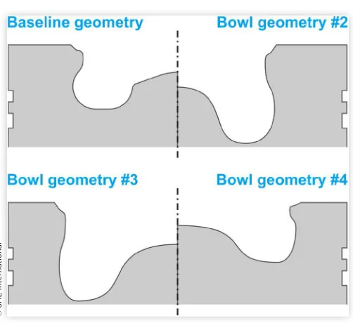
The generation of realistic and coherent combustion chamber designs was one of the most complex steps in this procedure. Chamber geometry can be very intricate which, in turn, complicates its recreation with only a few param-eters. Here, a piston bowl profile generator was implemented using Bezier polynomial curves and five optimizing param-eters [25]. As can be seen in Figure 5, this method offers a wide range of possible chamber designs, from large open bowls to tight and highly reentrant ones. The only restric-tion imposed on the chamber generarestric-tion was compression ratio, which was set to be the same as in the baseline case. The compression ratio was kept constant by adjusting the free squish height. However, in some cases where the
proposed geometry could not match the specified compres-sion ratio, it was discarded and a distinct set of random mutations were applied to the geometric parameters to generate a new one.
The two parameters considered to optimize the injector configuration were the spray inclusion angle to guide the fuel within the piston bowl, and the number of injector nozzle holes. In all cases, the total fuel mass injected, total nozzle area and injection pressure were kept constant. Therefore, nozzle diameter of the injector holes were adapted to maintain the overall injection area, assuming that the discharge coef-ficient remains constant for every hole. Therefore, the nozzle diameter was decreased as the number of nozzle holes were increased.
The design of intake ports was indirectly optimized by considering the swirl number at IVC as an optimizing param-eter in the GA loop. The magnitudes of the velocity compo-nents at initialization were accordingly adjusted so as to corre-spond to a given value of swirl number.
[image:7.612.310.561.93.323.2]The ranges of all the input parameters in the design space are listed in Table 4. These parameters and their ranges of variation were selected by taking into account possible tech-nological limitations such as minimum injector orifice diameter and maximum bowl depth.
TABLE 3 Summary of the constants and reference values in the merit function.
Parameter Eres ISFC NOx Soot
αi 3.0 2.0 -
-βi 2.0 2.0 -
-γi - - 15 0.5
xtarget 0.1 kPa2s 150 g/kWh -
-xlimit - - 7.54 mg/s 0.16 mg/s
© S A E I nt er na ti onal
FIGURE 5 Examples of different bowl profiles obtained by the Bezier polynomial method [25].
[image:7.612.65.293.147.226.2]© S A E I nt er na ti onal
TABLE 4 Ranges of the input parameters considered for GA optimization.
Geometric parameter 1 [-] 0.01-0.99 Geometric parameter 2 [-] 0.01-0.99 Geometric parameter 3 [-] 0.01-0.99 Geometric parameter 4 [-] 0.01-0.99 Geometric parameter 5 [-] 0.01-0.99 Number of injector nozzles [-] 4-12 Spray inclusion angle [deg] 80-180 Swirl number at IVC [-] 0.0-2.0
Results and Discussion
In this section, results from the optimization procedure are presented and discussed. First, the convergence of the GA is verified and trends of the output parameters are analyzed. Then, the comparison of the results between the simplified and original model setups is inspected. Finally, the outputs of the optimized configuration are compared against the baseline case and in-cylinder acoustic effects are analyzed in detail to understand the noise generation mechanisms.
Optimization Results
As the first step, algorithm convergence was verified to ensure that the GA reached a unique global optimum. Although convergence is mathematically determined since the mutation variability is reduced as the GA progresses, the attainment of the best solution after a given number of generations defined
a priori is not guaranteed. For this reason, the progression of the merit function as the GA progresses was tracked as shown in Figure 6. Besides the MF values for every simulation, the generation averaged value and the generation dispersion (±SD) are also included in the graph. It can be seen that the average
and dispersion are significantly reduced after the 12th
genera-tion (300th simulation). Nevertheless, the solution continues
to improve even after the 20th generation (500th simulation).
After this point, the average remains practically constant. The
dispersion however keeps oscillating until the 27th generation
(675th simulation), after which it becomes reasonably constant.
Observing this progress, the optimization was stopped after
the 29th generation and the GA was considered to
have converged.
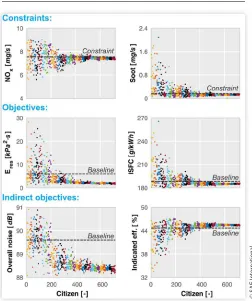
Subsequently, the inspection of the target and constraint parameters was carried out in order to check the solution success and compliance with the constraints. Figure 7 shows the progress of these parameters during the optimization
procedure. The graphs at the top show how both soot and NOx
emissions move towards their respective constraint values, reaching a final solution which practically coincides with these values. The middle graphs show notable improvements in both the objectives: while the energy of resonance is reduced by almost 70%, the ISFC exhibits an improvement of 2%. The bottom plots are included to illustrate how these improvements
affect the overall noise and indicated efficiency. It can be observed that noise emissions are reduced by acting directly on the resonance phenomena whereas the indicated efficiency is increased. This fact confirmed the suitability of this strategy for lowering noise emissions [56] as described in the previous section.
In addition to the general trends observed in these param-eters, in Table 5, a comparison between the baseline and opti-mized specifications is included to quantify the maximum improvement in all the relevant output parameters. As observed in the previous trends, the energy of resonance is lowered the most, so the overall noise is reduced by more than 1 dB. Moreover, indicated efficiency increases by 1.8%, whereas both pollutant emissions are maintained below their baseline levels.
FIGURE 6 Evolution of the merit function as the genetic algorithm progresses. An acceptable convergence is achieved after 29 generations.
©
S
A
E I
nt
er
na
ti
onal
FIGURE 7 Progress of objectives and constraints towards the optimum solution. The final targets (indirect objectives) of the optimization are also included.
©
S
A
E I
nt
er
na
ti
[image:8.612.313.565.297.598.2]onal
TABLE 5 Comparison between the baseline and optimized configurations. All relevant parameters are included to observe the changes in the main engine outputs.
Configuration Baseline Optimized
Eres [kPa2s] 5.95 1.53
ISFC [g/kWh] 188.3 184.9
NOx [mg/s] 7.54 7.48
Soot [mg/s] 0.16 0.12
Overall noise [dB] 89.6 88.2
Indicated eff. [%] 44.7 45.5 © SA
E I
nt
er
na
ti
© 2018 SAE International; Argonne National Laboratory.
The optimized configuration was further examined to determine which design parameters had changed to a greater extent. Hence, all the design parameters of both specifications are included in Figure 8 for comparison. The optimized geometry exhibits a deeper and tighter bowl profile with a less reentrant shape. The number of injector nozzle holes increases up to 12, as a result the nozzle diameter is also reduced. Finally, the spray inclusion angle is expanded by 13.4 degrees while the swirl number is slightly higher. These changes in the injector configuration and swirl would enhance the mixing rate and minimize spray penetration, thereby avoiding an excessive spray-wall impingement during the injection event.
Coherence of the Results
As mentioned in the previous section, certain modifications were made to the original model setup in order to reduce the computational time for the optimization. Although results of this modified model were considered sufficiently accurate since it captured the main trends of the original solution, the coherence of this solution must be verified by simulating the optimized system with the original model setup.
Therefore, a series of consecutive engine cycles using the optimized configuration were simulated with the original base mesh size (3 mm) and fixing the sonic Courant number to 1. As the design of the intake ports was indirectly optimized by the swirl number achieved after the gas exchange process, the velocity field was adjusted at IVC of each cycle to achieve the swirl number demanded by the optimized design. Following this approach, it was possible to modify the swirl motion during combustion without intake pressure changes, thereby
allowing a fair comparison between the two combustion systems. It was thus assumed that the new design reaches a high swirl with the same intake pressure.
The solution was considered converged after the third cycle, since the pressure trace and spectrum registered at the transducer location did not show any relevant dispersion.
Table 6 summarizes the results for the two model setups with both combustion system designs. It is evident how the simplified model causes the same effects on the solution in both designs. Every parameter which is overestimated in the baseline design (soot and indicated efficiency levels), is also overestimated in the optimized one, with the simplified model. In the same way, this behavior is also replicated in
every underestimated parameter (NOx and overall noise
levels). This fact evinces the consistency between both the numerical models, since they reproduce the trends even when the system configuration is completely modified.
Apart from this, the differences in NOx, soot and
effi-ciency levels between the two numerical models for the same engine configuration, show great similarity. For instance,
between the two numerical setups, NOx emissions vary by
0.33 mg/s for the baseline configuration whereas the difference for the optimized one is 0.37 mg/s.
However, this difference between the numerical setups is noticeably higher for noise levels. It is around 0.8 dB for the baseline, whereas in a case of the optimized configuration, a 1.6 dB of difference is seen. As Broatch et al. and Torregrosa et al. emphasized in several previous studies [22, 23, 56], local thermodynamic conditions before ignition govern the combustion phenomena and its subsequent in-cylinder pressure field effects. Therefore, limiting the simulation to the closed cycle and initializing the simulation with the results of the previous gas exchange process using the baseline config-uration, may affect the prediction of noise levels when the geometry is highly modified, since local thermodynamic conditions can change notably.
Despite this slight discrepancy, the simplified solution offers a good prediction of the main parameters and it achieves the optimization objective: It gives a combustion system configuration which reduces noise emissions while pollutant emissions and efficiency levels are maintained at the baseline level. Thus, even though not perfect in terms of prediction, the proposed approach is still a very reliable tool for incorpo-rating combustion noise of CDC in optimization methods.
Emissions Analysis
In this section, an analysis of pollutant emissions (NOx and
soot) is performed to understand the effect of the optimized FIGURE 8 Comparison of the baseline and optimized
configurations. Baseline bowl profile is plotted together with the optimized bowl geometry (top) whereas the injector and flow motion parameters are shown in the table (bottom).
©
S
A
E I
nt
er
na
ti
[image:9.612.48.299.118.374.2]onal
TABLE 6 Comparison of the predictions between the simplified and original model setups.
Setup Simplified model Original model
Configuration Baseline Optim. Baseline Optim.
NOx [mg/s] 7.54 7.48 7.87 7.85
Soot [mg/s] 0.16 0.12 0.13 0.10
Overall noise [dB] 89.6 88.2 90.4 89.8 Indicated eff. [%] 44.7 45.5 42.7 43.6
©
S
A
E I
nt
er
na
ti
combustion system design. This study uses the solutions of the original model setup (base mesh size of 3 mm) to increase the integrity of the results and therefore the soundness of the conclusions.
Although emissions levels are practically the same in both specifications, it does not necessarily imply that they evolve in the same way during the cycle. Consequently, the produc-tion and later oxidaproduc-tion of these pollutants may change. For instance, Figure 9 (top) shows how soot mass follows different paths as the combustion progresses. The maximum amount of soot is clearly lower in the optimized configuration. This indicates that the optimized design enhances in-cylinder mixing, thereby lowering soot production.
In Figure 9 (bottom), the fuel mass versus equivalence ratio is shown at 24 CAD aTDC. It can be clearly seen that the
fuel mass within the soot production region (ϕ > 2) is
substan-tially decreased for the optimized case as compared to the baseline, thereby leading to lower soot production. Nonetheless, the optimized design is not able to oxidize the same amount of soot as the baseline, reaching nearly the same levels of soot at the end of the closed cycle. This particular behavior is probably caused by the shortage of oxygen within the optimized piston bowl due to its extremely deep design.
On the other hand, as can be seen in Figure 10, NOx
emis-sions barely exhibit differences between the two configura-tions. Only slight differences can be observed during the combustion of the two pilot injections.
Acoustic Analysis
In addition to consider combustion noise control in optimiza-tion strategies, another important aspect of this investigaoptimiza-tion is to reproduce the pressure oscillations that are present in a real engine and are responsible for resonant combustion noise. The comprehension of such complex phenomena is critical to devise strategies for combustion noise mitigation.
The numerical pressure data available from the simula-tions, once validated, can then be analyzed through different techniques to reveal the real behavior of the in-cylinder pressure field, thus providing valuable information about pressure oscillation modes, their characteristic frequencies and their temporary evolution. However, the complexity of the resonant acoustic field complicates even a simple recre-ation for visualizrecre-ation purposes and hinders a correct inter-pretation of the involved phenomena.
For this reason, most of acoustics related studies till date have focused on performing basic and straightforward analyses which are based on qualitative comparisons of the acoustic field [57] or traditional acoustic metrics [58]. Only a few of them attempted to link the frequency content with the spatial energy distribution [23] or the time evolution [59], in an effort to understand the propagation and dissipation patterns.
A way to explore the spatial distribution of the acoustic pressure field for different frequency phenomena of interest is to perform Fast Fourier Transform (FFT) at each cell record in the considered domain. Then, the dispersion of the high frequency spectra gives an idea, at least in a qualitative way, about the variability of the pressure field in the combustion chamber. Figure 11 exemplifies this procedure; the averaged pressure spectra are plotted together with the spatial variation, represented by the standard deviation (±SD), for both configu-rations considered so far. Interesting information can be obtained about the most excited modes from this comparison. It appears that the acoustic energy is shifted towards higher frequencies for the optimized configuration. Consequently, new resonant modes experience a notable lowering of ampli-tude, causing the reduction of the overall resonant noise. Also, the spatial variability is reduced in the frequencies for which the modes are attenuated (6-8.5 kHz) and, conversely, it is FIGURE 9 Soot mass evolution versus crank angle for both
baseline and optimized configurations (top). Analysis of local conditions evaluated at 24 CAD aTDC. Fuel mass versus equivalence ratio is also included for both
configurations (bottom).
©
S
A
E I
nt
er
na
ti
onal
FIGURE 10 NOx mass as a function of the crank angle for
both combustion system configurations: baseline and optimized.
©
S
A
E I
nt
er
na
ti
© 2018 SAE International; Argonne National Laboratory.
increased at the harmonics with higher level of excitation (8.5-13 kHz and 15-20 kHz).
Although this information sheds some light on the in-cylinder pressure field, it becomes impossible to imagine how this field is locally changing, given the limitations of this method. Some studies have taken a step forward by combining FFT, band-pass filtering and multiple monitor points in the combustion chamber [21] in order to overcome these limita-tions. However, they still missed the temporal evolution of each acoustic mode. In this context, proper orthogonal decomposi-tion (POD), also known as principal component analysis (PCA) or Karhunen-Loève expansion [60, 61], is a viable tool suitable for identifying which spatial structures comprise most of the energy of the flow field. This method decomposes the flow into both spatial and temporal orthogonal modes whereas frequency components of these modes can be obtained by FFT application. Thus, once the method is applied, a complete connection between spatial, temporal and frequency domains can be revealed. Although some studies have specifically addressed ICE combustion issues through POD, they have been focused on cycle-to-cycle variation analysis [62, 63], spark-ignition engine misfire [64] or the evolution of a particular species [65]. Only Torregrosa et al. [66] have applied this method to acoustic issues of combustion chambers.
Taking the previous work by Torregrosa et al. [66] as a reference, a POD analysis of the in-cylinder pressure field was carried out to address the limitations of previous methods
mentioned above. Orthonormal POD modes (Ψi) and their
corresponding energy of excitation (obtained from their
prin-cipal values σi) were obtained, together with the temporal
evolution coefficients (ai).
In order to characterize the relevance of each mode, its contribution to the total resonance energy was analyzed, as shown in the Pareto charts of Figure 12. It can be seen that
the POD modes Ψ1-11 gather approximately 70% of the
resonant energy, with 50% being gathered just by modes Ψ1-5.
Although not shown in the figure, 80% of the remaining
energy is represented by modes Ψ1-26 and finally modes Ψ1-179
sum up to 99%. The rest of the modes represent just 1% of the remaining energy. Apart from that, for the baseline
configuration, the first three modes (Ψ1-3) account for the
major part of this energy while the energy distribution for the optimized configuration is more equitable.
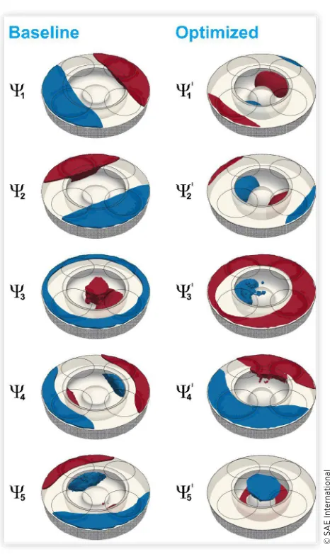
The pressure amplitude associated with each set of coor-dinates is plotted in Figure 13 using a set of iso-volumes. POD
modes Ψ1-5 are thus displayed by showing the upper and lower
10% tails (i.e., the 10% and 90% percentiles) of the distribution of their amplitudes. In this figure, red and blue volumes thus indicate the distribution of the top 10% positive and negative amplitudes of the mode. In other words, the red and blue volumes identify the regions oscillating with alternating higher amplitudes. On the other hand, the nodal regions whose amplitude remains mostly constant in time, correspond to the empty volume regions. The five most energetic modes were included in the analysis since they exhibited the most meaningful differences between the two designs.
Inspecting the shapes of modes Ψ1 and Ψ2 in Figure 13,
it can be clearly observed how the higher amplitudes are oscil-lating on opposite sides of the squish zone, in two different orientations. Furthermore, these two modes are reminiscent of the classical acoustic transversal modes in open combustion chambers, specifically mode (m = 1, n = 0) in the notation of Hickling et al. [21], also called the first asymmetric mode. In
contrast to these, POD mode Ψ3 features a completely circular
distribution between the squish zone and the bowl, with an annular nodal region instead of a straight one like in the previous modes, being similar to Hickling’s first radial mode (m = 0, n = 1).
FIGURE 11 Comparison of the in-cylinder pressure spectra trends. The pressure spectrum averaged over all cells in the domain is plotted with its standard deviation (±SD) for both configurations (baseline and optimized).
©
S
A
E I
nt
er
na
ti
onal
FIGURE 12 Pareto charts showing the energy contributions of POD modes Ψ1-11 and the accumulated contribution to the
resonance energy in each configuration: the baseline (top) and the optimized (bottom).
©
S
A
E I
nt
er
na
ti
There is another interesting aspect in Figure 13 which can provide additional information about the resonant modes’ behavior. It can be seen how the spatial distribution of the most energetic modes are remarkably different in both engine configurations.
[image:12.612.62.295.129.520.2]Recalling the energy distribution of the modes plotted in Figure 12, the energy share and spatial distribution of POD
modes Ψ’
1-5 are plotted in Figure 14, along with the
corre-sponding most closely resembling modes of the baseline (Ψ1,3,4,5,8). This figure shows how the modal energy has shifted
from the original to the modified combustion, i.e., how the spatial distribution of the unsteady pressure fluctuations has been affected by the change in engine design. It can be seen
that Ψ’
1-2 modes which were previously ranked fourth and
fifth with 5.36% and 3.48% of the energy, are now the most relevant with an energy share of 17.73% and 13.57%,
respec-tively. Modified mode Ψ’
3 is found to closely resemble the
original Ψ3 mode. Its energy content, on the other hand, has
been slightly diminished. Finally, mode Ψ8 for the original
bowl has been promoted to the fifth place for the optimized configuration, with almost three times its previous energy. Therefore, it is possible to claim that the transfer of resonant energy to higher frequencies, which was observed in Figure 11, is also accompanied by a change in the spatial distribution of the pressure field.
The information contained within the POD data also allows the analysis of the evolution of each mode in time and frequency domains. In Figure 15, the frequency content
asso-ciated to Ψ1,4,8 and Ψ’4,1,5 modes is presented. It is evident that
each POD mode is associated with a specific frequency band. These modes were specifically selected to illustrate the effects
described in Figure 11. For instance, modes Ψ1 and Ψ’4 clearly
mimic the reduction of the pressure spectra gathered between 5 and 8.5 kHz. In a similar way, the rest of the represented modes aim to reproduce the energy increase observed for the frequencies comprising 8.5-13 kHz and 15-20 kHz. Again, this clearly depicts how the pressure field changes its spatial
FIGURE 13 Spatial distributions of the POD modes Ψ1-5
across the simulated combustion chamber. Each mode is represented by colored iso-volumes indicating the 10% (blue) and 90% (red) percentiles of the distribution of the real values of each individual mode.
©
S
A
E I
nt
er
na
ti
onal
FIGURE 14 Energy share and spatial distribution of the five most relevant optimized design modes Ψ’
1-5
(top), together with their most closely resembling baseline counterparts (bottom).
©
S
A
E I
nt
er
na
ti
onal
FIGURE 15 Normalized amplitudes of POD modes Ψ1,4,8
and Ψ’
4,1,5 in the frequency domain.
©
S
A
E I
nt
er
na
ti
© 2018 SAE International; Argonne National Laboratory.
distribution as the frequencies being excited vary. On the other hand, it is interesting to note that the energy of the modes is progressively concentrated within the bowl as the frequency increases, going from completely squish-dominated modes at 5-8.5 kHz to entirely inside-bowl oscillations at 15-20 kHz. Meanwhile a mixed effect of both is easily identifi-able at 8.5-13 kHz.
Continuing this comparison, Figure 16 displays the time evolution of these three specific modes, in an attempt to find possible relationships between the inception of these modes and different phases of the combustion process. The first plot
depicts how the onset of mode Ψ1 is coincident with the start
of combustion of the first pilot. Moreover, the amplitude rapidly reaches its maximum value during the second pilot
combustion phase. This mode is again excited during the diffusive combustion, with its amplitude increasing practically
up to the highest value. Mode Ψ’
4 however, starts to develop
after the onset of the second combustion phase and practically disappears very soon after the start of the third combustion stage. This indicates the relevance of the early pilot injections in the resonant noise generation, since they heavily contribute to the excitation of less energetic modes.
In the second plot, both modes Ψ4 and Ψ’1 appear at the
second ignition event, although the amplitude rise is much
more pronounced for mode Ψ’
1 while for mode Ψ4 the time
evolution is essentially constant during the whole combustion.
Furthermore, the amplitude of mode Ψ’
1 increases during the
main combustion stage, reaching its maximum value at 10 CAD aTDC.
Finally, the last plot shows the evolution of Ψ8 and Ψ’5
modes. Mode Ψ’
5 displays an amplitude rise at the start of the
last two combustion phases but its intensity is severely attenu-ated due to its high characteristic frequencies. On the other
hand, mode Ψ8 shows little relevance after the second
combus-tion onset, only exhibiting a significant amplitude during this short stage.
Summary and Conclusions
In this paper, a numerical methodology for combustion system optimization of an internal combustion engine was proposed, with the target of controlling combustion noise while maintaining (or even improving) pollutant emissions and performance. The methodology was based on the combi-nation of genetic algorithm method and CFD modeling, specifically implemented to accurately assess the source of combustion noise emissions. Special attention was given to recreation of the frequency response of the pressure field within the combustion chamber.This methodology was employed to optimize the combustion system of a CI diesel engine considering chamber geometry, injector specifications and in-cylinder swirl, in order to promote a quieter engine design by mini-mizing high frequency pressure oscillations. The new system was able to reduce noise emissions, owing to the lowering of resonance energy, since it modified the frequency content to feature higher frequencies, less perceptible by human hearing.
The optimized design included a deeper and tighter bowl geometry with higher swirl and greater number of nozzle holes with smaller nozzle diameters. The changes in the injector and swirl led to enhanced mixing rate and mini-mized spray penetration, thereby avoiding excessive spray-wall impingement during the injection event. Moreover, the spray inclusion angle increased in order to match with the new bowl geometry.
In addition, a detailed analysis of the in-cylinder acoustic effects was carried out to understand the unsteady pressure field behavior and to identify the most relevant noise issues. POD decomposition of the results for both the baseline and optimized designs was performed, revealing the energy shifting between modes as a result of the different combustion
FIGURE 16 Normalized amplitudes of the POD modes Ψ1,4,8
and Ψ’
4,1,5 in time domain. The different
combustion phases are also identified to connect possible combustion features with temporary changes in the time evolution of each mode.
©
S
A
E I
nt
er
na
ti
system features. The most dominant mode, and thus the main source of resonant emissions, was significantly attenuated whereas the amplitudes of higher order modes were accord-ingly increased, albeit never reaching levels as high as the first one. Besides the frequency shift, the pressure field also expe-rienced a change in spatial distribution. Specifically, the spectral content at 5-8.5 kHz was related to the squish- dominated pulsation, the 8.5-13 kHz frequencies featuring squish-bowl interaction and the higher frequency content at 15-20 kHz related to central top-down bowl oscillations. Finally, a relation between the inception of the modes and different phases of the combustion was identified, showing how early pilot injections significantly contributed to the exci-tation of less energetic modes.
In summary, the methodology presented in this work allowed identification of an optimization path for dimin-ishing combustion noise, by acting on the acoustic source. The subsequent acoustic analysis provided a detailed under-standing of the resonant pressure oscillations within the combustion chamber. Interestingly, the optimization meth-odology and analytical tools employed in this study are quite general and can be readily applied to different engine config-urations and combustion concepts (such as knock in spark-ignited engines [67, 68]), which will be explored as part of future work.
References
1. Kampa, M. and Castanas, E., “Human Health Effects of Air Pollution,” 4th International Workshop on Biomonitoring of Atmospheric Pollution 151(2):362-367, 2008, doi:10.1016/j. envpol.2007.06.012.
2. “szCDP Global Climate Change Report 2015,” Carbon Disclosure Project, 2015.
3. Hasegawa, R. and Yanagihara, H., “HCCI Combustion in DI Diesel Engine,” SAE Technical Paper 2003-01-0745, 2003, doi:10.4271/2003-01-0745.
4. Hardy, W. L. and Reitz, R. D., “A Study of the Effects of High EGR, High Equivalence Ratio, and Mixing Time on Emissions Levels in a Heavy-Duty Diesel Engine for PCCI Combustion,” SAE Technical Paper 2006-01-0026, 2006, doi:10.4271/2006-01-0026.
5. Dec, J.E., “Advanced Compression-Ignition Engines-Understanding the in-Cylinder Processes,” Proceedings of the Combustion Institute 32(2):2727-2742, 2009, doi:10.1016/j. proci.2008.08.008.
6. Hanson, R., Splitter, D., and Reitz, R. D., “Operating a Heavy-Duty Direct-Injection Compression-Ignition Engine with Gasoline for Low Emissions,” SAE Technical Paper 2009-01-1442, 2009, doi:10.4271/2009-01-1442.
7. Manente, V., Johansson, B., Tunestal, P., and Cannella, W., “Effects of Different Type of Gasoline Fuels on Heavy Duty Partially Premixed Combustion,” SAE Int. J. Engines 2(2):71-88, 2010, doi:10.4271/2009-01-2668.
8. Masterton, B., Heffner, H., and Ravizza, R., “The Evolution of Human Hearing,” The Journal of the Acoustical Society of America 45(4):966-985, 1969, doi:10.1121/1.1911574.
9. Schwarz, A. and Janicka, J., “Combustion Noise,” (Berlin, Springer-Verlag, 2009).
10. Strahle, W.C., “Combustion noise,” Progress in Energy and Combustion Science 4(3):157-176, 1978, doi:10.1016/0360-1285(78)90002-3.
11. Flemming, F., Sadiki, A., and Janicka, J., “Investigation of Combustion Noise Using a LES/CAA Hybrid Approach,”
Proceedings of the Combustion Institute 31(2):3189-3196, 2007, doi:10.1016/j.proci.2006.07.060.
12. Ren, Y., Randall, R.B., and Milton, B.E., “Influence of the Resonant Frequency on the Control of Knock in Diesel Engines,” Proceedings of the Institution of Mechanical Engineers, Part D: Journal of Automobile Engineering
213(2):127-133, 1999, doi:10.1243/0954407991526748. 13. Torregrosa, A.J., Broatch, A., Martín, J., and Monelletta, L.,
“Combustion Noise Level Assessment in Direct Injection Diesel Engines by Means of in-Cylinder Pressure Components,” Measurement Science and Technology
18(7):21-31, 2007, doi:10.1088/0957-0233/18/7/045.
14. Payri, F., Broatch, A., Margot, X., and Monelletta, L., “Sound Quality Assessment of Diesel Combustion Noise Using in-Cylinder Pressure Components,” Measurement Science and Technology 20(1):01-12, 2009,
doi:10.1088/0957-0233/20/1/015107.
15. Payri, F., Torregrosa, A.J., Broatch, A., and Monelletta, L., “Assessment of Diesel Combustion Noise Overall Level in Transient Operation,” International Journal of Automotive Technology 10(6):761, 2009, doi:10.1007/s12239-009-0089-y. 16. Stanković, L. and Böhme, J.F., “Time-Frequency Analysis of
Multiple Resonances in Combustion Engine Signals,” Signal Processing 79(1):15-28, 1999,
doi:10.1016/S0165-1684(99)00077-8.
17. Singh, O.P., Sreenivasulu, T., and Kannan, M., “The Effect of Rubber Dampers on engine’s NVH and Thermal
Performance,” Applied Acoustics 75:17-26, 2014, doi:10.1016/j. apacoust.2013.07.007.
18. Anderton, D., “Relation between Combustion System and Engine Noise,” SAE Technical Paper 790270, 1979, doi:10.4271/790270.
19. Liu, H., Zhang, J., Guo, P., Bi, F. et al., “Sound Quality Prediction for Engine-Radiated Noise,” Mechanical Systems and Signal Processing 56:277-287, 2015, doi:10.1016/j. ymssp.2014.10.005.
20. Vressner, A., Lundin, A., Christensen, M., Tunestål, P. et al., “Pressure Oscillations during Rapid HCCI Combustion,” SAE Technical Paper 2003-01-3217, 2003, doi:10.4271/2003-01-3217.
21. Hickling, R.F.D.A. and Sung, S.H., “Knock-Induced Cavity Resonances in Open Chamber Diesel Engines,” Acoustic Society of America 65(5):1474-1479, 1979, doi:10.1121/1.382910. 22. Broatch, A., Margot, X., Novella, R., and Gomez-Soriano, J.,
“Combustion Noise Analysis of Partially Premixed Combustion Concept Using Gasoline Fuel in a 2-Stroke Engine,” Energy
107:612-624, 2016, doi:10.1016/j.energy.2016.04.045.
© 2018 SAE International; Argonne National Laboratory.
24. Torregrosa, A.J., Broatch, A., Margot, X., and Marant, V., “Combustion Chamber Resonances in Direct Injection Automotive Diesel Engines: A Numerical Approach,”
International Journal of Engine Research 5(1):83-91, 2003, doi:10.1243/146808704772914264.
25. Benajes, J., Novella, R., Pastor, J.M., Hernández-López, A. et al., “Optimization of the Combustion System of a Medium Duty Direct Injection Diesel Engine by Combining CFD Modeling with Experimental Validation,” Energy Conversion and Management 110:212-229, 2016, doi:10.1016/j.
enconman.2015.12.010.
26. Hiroyasu, H., Miao, H., Hiroyasu, T., Miki, M. et al., “Genetic Algorithms Optimization of Diesel Engine Emissions and Fuel Efficiency with Air swirl, EGR, Injection Timing and Multiple Injections,” SAE Technical Paper 2003-01-1853, 2003, doi:10.4271/2003-01-1853.
27. Costa, M., Bianchi, G.M., Forte, C., and Cazzoli, G., “A Numerical Methodology for the Multi-Objective
Optimization of the DI Diesel Engine Combustion,” Energy Procedia 45:711-720, 2014, doi:10.1016/j.egypro.2014.01.076. 28. Park, S.W., “Optimization of Combustion Chamber
Geometry for Stoichiometric Diesel Combustion Using a Micro Genetic Algorithm,” Fuel Processing Technology
91(11):1742-1752, 2010, doi:10.1016/j.fuproc.2010.07.015. 29. Wickman, D., Yun, H., and Reitz, R., “Split-Spray Piston
Geometry Optimized for HSDI Diesel Engine Combustion,” SAE Technical Paper 2003-01-0348, 2003, doi:10.4271/2003-01-0348.
30. Senecal, P. and Reitz, R., “Simultaneous Reduction of Engine Emissions and Fuel Consumption Using Genetic Algorithms and Multi-Dimensional Spray and Combustion Modeling,” SAE Technical Paper 2000-01-1890, 2000, doi:10.4271/2000-01-1890.
31. Sun, Y., Wang, T., Lu, Z., Cui, L. et al., “The Optimization of Intake Port using Genetic Algorithm and Artificial Neural Network for Gasoline Engines,” SAE Technical Paper 2015-01-1353, 2015, doi:10.4271/2015-01-1353.
32. Payri, F., Olmeda, P., Martín, J., and García, A., “A Complete 0D Thermodynamic Predictive Model for Direct Injection Diesel Engines,” Applied Energy 88(12):4632-4641, 2011, doi:10.1016/j.apenergy.2011.06.005.
33. CONVERGENT SCIENCE Inc., “CONVERGE 2.2 Theory Manual,” 2015.
34. Ihlenburg, F., “The Medium-Frequency Range in
Computational Acoustics: Practical and Numerical Aspects,”
Journal of Computational Acoustics 11(02):175-193, 2003, doi:10.1142/S0218396X03001900.
35. Yakhot, V. and Orszag, S., “Renormalization Group Analysis of Turbulence,” Journal of Scientific Computing 1(1):3-51, 1986, doi:10.1007/BF01061452.
36. Angelberger, C., Poinsot, T., and Delhay, B., “Improving Near-Wall Combustion and Wall Heat Transfer Modeling in SI Engine Computations,” SAE Technical Paper 972881, 1997, doi:10.4271/972881.
37. Redlich, O. and Kwong, J.N., “On the Thermodynamics of Solutions. V. An Equation of State. Fugacities of Gaseous Solutions,” Chemical Reviews 44(1):233-244, 1949, doi:10.1021/cr60137a013.
38. Issa, R., “Solution of the Implicitly Discretised Fluid Flow Equations by Operator-Splitting,” Journal of Computational Physics 62:40-65, 1986, doi:10.1016/0021-9991(86)90099-9. 39. Dukowicz, J.K., “A particle-fluid numerical model for liquid
sprays,” Journal of Computational Physics 35(2):229-253, 1980, doi:10.1016/0021-9991(80)90087-X.
40. Reitz, R.D. and Beale, J.C., “Modeling Spray Atomization with the Kelvin-Helmholtz/Rayleigh-taylor Hybrid Model,”
Atomization and Sprays 9(6):623-650, 1999, doi:10.1615/ AtomizSpr.v9.i6.40.
41. O’Rourke, P.J., “Collective Drop Effects on Vaporizing Liquid Sprays,” Ph.D. thesis, Princeton University, 1981. 42. Amsden, A. A., O’Rourke, P. J., and Butler, T. D., “KIVA-II:
A Computer Program for Chemically Reactive Flows with Sprays,” Los Alamos National Laboratory Report No. LA-11560-MS, 1989.
43. Liu, A.B., Mather, D.K., and Reitz, R.D., “Modeling the Effects of Drop Drag and Breakup on Fuel Sprays,” SAE Paper No. 930072, 1993, doi:10.4271/930072.
44. Brakora, J. and Reitz, R., “A Comprehensive Combustion Model for Biodiesel-Fueled Engine Simulations,” SAE Technical Paper 2013-01-1099, 2013, doi:10.4271/2013-01-1099.
45. Hiroyasu, H. and Kadota, T., “Models for Combustion and Formation of Nitric Oxide and Soot in Direct Injection Diesel Engines,” SAE Technical Paper 760129, 1976, doi:10.4271/760129.
46. Heywood, J.B., “Internal Combustion Engine Fundamentals,” (McGraw-Hill Inc, 1998).
47. Senecal, P., Pomraning, E., Richards, K., Briggs, T. et al., “Multi-Dimensional Modeling of Direct-Injection Diesel Spray Liquid Length and Flame Lift-off Length using CFD and Parallel Detailed Chemistry,” SAE Technical Paper 2003-01-1043, 2003, doi:10.4271/2003-01-1043.
48. Babajimopoulos, A., Assanis, D.N., Flowers, D.L., Aceves, S.M. et al., “A Fully Coupled Computational Fluid Dynamics and Multi-Zone Model with Detailed Chemical Kinetics for the Simulation of Premixed Charge Compression Ignition Engines,” International Journal of Engine Research 6(5):497-512, 2005, doi:10.1243/146808705X30503.
49. Pal, P., Keum, S., and Im, H.G., “Assessment of Flamelet Versus Multi-Zone Combustion Modeling Approaches for Stratified-Charge Compression Ignition Engines,”
International Journal of Engine Research 17(3):280-290, 2016, doi:10.1177/1468087415571006.
50. Pal, P., “Computational Modeling and Analysis of Low Temperature Combustion Regimes for Advanced Engine Applications”, Ph.D. Dissertation, University of Michigan-Ann Arbor, 2016, http://hdl.handle.net/2027.42/120735. 51. Pickett, L., Bruneaux, G., and Payri, R., Engine Combustion
Netwrok, 2014.
52. Pal, P., Probst, D., Pei, Y., Zhang, Y. et al., “Numerical Investigation of a Gasoline-like Fuel in a Heavy-Duty Compression Ignition Engine Using Global Sensitivity Analysis,” SAE Int. J. Fuels Lubr. 10(1), 2017,
doi:10.4271/2017-01-0578.