Temporal Spatial Consistency and Sampling Neural Network Based Adaptive Hand held Video Deblurring

2019 International Conference on Information Technology, Electrical and Electronic Engineering (ITEEE 2019) ISBN: 978-1-60595-606-0

Temporal-Spatial Consistency and Sampling Neural Network

Based Adaptive Hand-held Video Deblurring

Xiao LI

, Shuai LI

, Hong QIN

and Ai-min HAO

1_{State Key Laboratory of Virtual Reality Technology and Systems, Beihang University,} Beijing, 100191, China

2_{Beihang University Qingdao Research Institute, Qingdao, 266000, China} 3_{Department of Computer Science, Stony Brook University, New York, 11794, USA}

*Corresponding author

Keywords: Neural network, Adaptive video deblurring, Temporal alignment, Spatial consistency alignment, Luckiness threshold value.

Abstract. Video deblurring for hand-held camera is vital in many high-level video enhancement applications. Although quite a few proposed approaches have achieved remarkable success in recent years, many technical challenges still prevail for video (from hand-held camera) containing wide-range scenes and highly-variable objects. In particular, we are lacking effective and versatile strategies to adaptively handle high-level alignment, parallax diminution, unclear area detection, sharpness enhancement in a consistent fashion. To ameliorate, this paper develops a novel method to successively respect temporal-spatial alignment and precise deblurring. Our aim is to devise a new adaptive video deblurring technique by resorting to new modeling strategies. This paper's key originality is hinged upon the joint utility of both self-adaptive intrinsic mode functions (IMFs) based on empirical mode decomposition (EMD) in the temporal domain for video signal and mesh-structure constraint enforcement in the spatial domain, beside, this paper innovatively jointly utilities the subsampling convolution, upsampling convolution and luckiness threshold value based back propagation, which takes video deblurring as a high-precision adaptive convolution. As a result, our new approach can adaptively improve the clarity of the video, and synchronously optimize the camera trajectory of wobbly video. To validate our optimization approach for adaptive video deblurring, we conduct comprehensive experiments on public benchmarks, and make extensive and quantitative evaluations with available state-of-the-art methods as well as popular commercial software. All of our experiments demonstrate the advantages of the optimization method in terms of versatility, accuracy, and efficiency.

Introduction and Motivation

First, from the perspective of producing a stable parallax-free camera trajectory based on saliency preservation, the parallax caused by non-trivial depth variation in the scene makes the image deblurring become an ill-posed problem, because different regions may require different trajectories and spatially-variant homographies. Although spatial multidimensional reconstruction can deal with the parallax in principle and generate more stable results, however, multidimensional motion model estimation is far less robust due to various degenerations and frequently ignores the conservation of saliency features. Therefore, how to simultaneously exploit the spatially-variant homographies to produce a uniform parallax-free temporal-spatial consistency homography based on saliency preservation is urgently needed in video deblurring.

Second, from the perspective of removing unambiguous pixels generating sharp pixels adaptively, current methods more or less suffer from the following problems. It is difficult to handle more challenging cases (e.g., rapid motion, fast scene transition, large occlusion) by straightforwardly removing unambiguous areas without sufficient self-adaptation, because the camera motion tends to have an intrusive nature under some circumstances. Thus, considering the optimizing quality of original video, how to design adaptive deblurring model to analyze and deblur the shaking video, is extremely essential for the robust and high-quality result.

Third, from the perspective of iteratively improving video clarity, current methods more or less suffer from the following problems. Lots of techniques pay too much attention to deblurring local region and ignore protecting the original appearance of the video. Thus, considering iteratively improving the clarity of unsharp video, it needs an accurate but simple strategy to flexibly detect the clarity of overall video.

To tackle the aforementioned challenges, we shall concentrate on the self-adaptive video deblurring by taking full advantages of both deconvolution and fusion methods. Specifically, our salient contributions can be summarized as follows:

We propose a homography estimation method of temporal-spatial structure consistency with preserving salient image regions, which gives rise to the efficient and effective revealing of the intrinsic motion consistence among different regions in wobbly video.

We propose a self-adaptive upsampling and subsampling convolution based on Neural Network, which can make the shaking video be more sharp, and also facilitate the analysis and optimization of blurry videos.

We propose a back propagation strategy based on luckiness threshold value, which can iteratively improve the clarity of the video, while maintaining the original appearance of the video.

Related Works

Deconvolution Based Deblurring

The above methods tend to be more fragile and often introduce unwanted artifacts such as ringing and amplified noise because of the strong dependence on the accuracy of the assumed image degradation model.

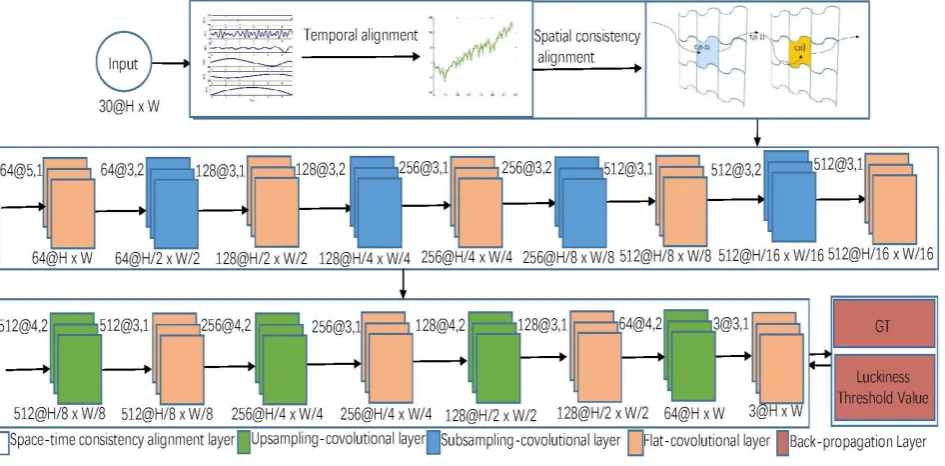
Figure 1. Architecture of the proposed deblurring model with four stages, which consisting of space-time consistency alignment module, subsampling-convolutional module, upsampling-convolutional module, and back-propagation module, takes the nearby 10 frames as input. Each frame includes red, green and blue color parameters. The second stage contains four pairs combination of flat-convolutional layer and the subsampling layer. The third stage contains four pairs combination of flat-convolutional layer and the upsampling convolutional layer. Each of convolutional layer

includes the filter bank module, batch normalization and a nonlinear module with a relu activation function.

Fusion Based Deblurring

Image fusion method produces a single image from a set of input images. The fused image should have more complete information which is more useful for human or machine perception. This single image is more informative and accurate than any single source image, and it consists of all the necessary information. The purpose of image fusion is not only to reduce the amount of data but also to construct images that are more appropriate and understandable for the human and machine perception[1]. Joshi et al.[6] use a novel local weighted averaging method based on ideas from “lucky imaging” to minimize blur, resampling and alignment errors, as well as effects of sensor dust, to maintain the sharpness of the original pixel grid. Law et al.[8] use a Lucky Imaging system to obtain I-band images with much improved angular resolution on a ground-based 2.5m telescope. Instead of estimating point spread functions, Matsushita et al.[12] transfer and interpolate sharper image pixels of neighboring frames to increase the sharpness of the frame to deblur the target frame. Delbracio et al.[3] present an algorithm that removes blur due to camera shake by combining information in the Fourier domain from nearby frames in a video.

All above methods are limited by their computation and evaluation, which is not reliable in some complicated situations, such as occlusions and outliers.

Neural Network Based Deblurring

learning to achieve further improved results. Iizuka et al.[5] feature a fusion layer to elegantly merge local information dependent on small image patches with global priors computed using the entire image. Pathak et al.[16] propose Context Encoders – a convolutional neural network trained to generate the contents of an arbitrary image region conditioned on its surroundings.

However, the above methods address different problems, with different sets of challenges. This paper focuses on deblurring, where blurry frames can vary greatly in appearance from their neighbors, making information fusion more challenging. We propose a subsampling-convolution and upsampling-convolution neural network for video deblurring, using synthetic training data.

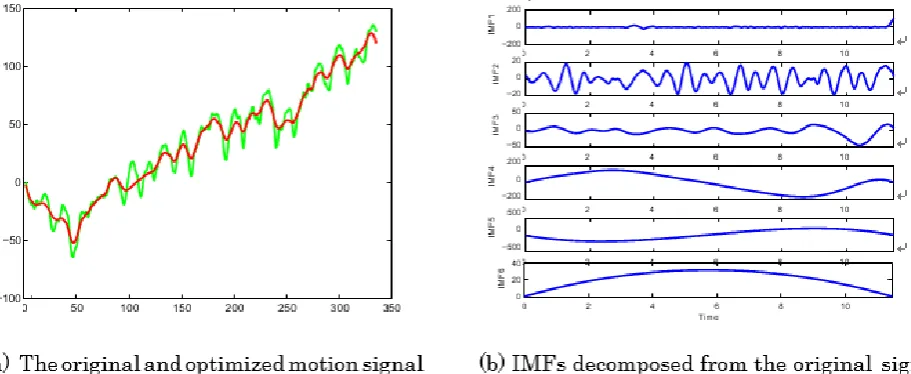
Figure 2. (a) The green line denotes the original signal before smoothing, and the red line denotes the optimized motion signal after smoothing by Eq. (4). (b) The IMF signals decomposed from the original signal.

Method Overview

Our architecture. With limited training shapes, the depth of our architecture should not be very complex, otherwise with the growth of layer number, the parameters would rapidly increase so as to produce overfit. Thus, the structure consists of four major stages. As shown in Fig. 1, in our approach, four modules are proposed, which are space-time consistency alignment module, subsampling-convolutional module, upsampling-convolutional module, and back-propagation module. The nearby 10 frames including the unsharp frame are taken as input. Each frame includes three parameters which are red, green and blue parameter. So the number of our input is 30. The output is a deblurred center frame in the jacent 10 frames.

Image alignment is inherently challenging for video deblurring, as it may be very difficult to use low-level features to determine whether aligned pixels in different images correspond to the same scene content. Advanced features, on the other hand, provide enough additional information to help separate areas of the image that are not properly aligned from the correctly aligned image area. In order to utilize both low-level and high-level features, we have presented a space-time consistency alignment module, which includes self-adaptive IMFs based temporal alignment and saliency preserving based spatial consistency alignment. Subsampling-convolutional module consists of four pairs combination of flat-convolutional layer and the subsampling convolutional layer. The flat convolutional module is for non-linear mapping and preserve the size of the image. Upsampling-convolutional module consists of four pairs combination of flat-convolutional layer and the upsampling convolutional layer. The flat convolutional module is for non-linear mapping and preserve the size of the image. Back-propagation module uses MSE to the ground truth sharp image and luckiness threshold value, which greatly improves the sharpness of the image.

Space-time Consistency Alignment Module

Self-Adaptive IMFs Based Temporal Alignment

SIFT Based Homography Construction. Using the method proposed by Lowe et al.[11], we frame-wisely extract the SIFT features from the wobbly video. From the SIFT features, we can get the descriptor component and the location component. One SIFT match is accepted only if its Euclidean distance is less than 𝑑𝑖𝑠𝑡𝑅𝑎𝑡𝑖𝑜 times the distance to the second closest match. Generally, we set 𝑑𝑖𝑠𝑡𝑅𝑎𝑡𝑖𝑜 as 0.1. The Euclidean distance from the previous point to the next point is the length of the line segment connecting them.

Through the above process, the 𝑀 × 2 matrices of [x,y] coordinates can be obtained. Outliers in matched points of two frames are excluded by using M-estimator SAmple Consensus (MSAC) algorithm[23]. The geometric transformation maps the inliers in matched points of the last frame to the inliers in those of the next frame. Using geometric transformation algorithm[14], we could compute and denote the geometric transformation with the 3 × 3 matrix 𝑇_𝑡:

𝑇_𝑡 = [𝑅𝑡 𝑂𝑡

0 1]. (1) In Eq. (1), 𝑅_𝑡 and 𝑂_𝑡 are the 2 × 2 rotation matrix and 2 × 1 translation vectors, representing the camera motion orientation and position in the global coordinate system respectively.

As shown in Fig. 3, we denote camera pose at frame t as 𝑆_𝑡. The relative camera motion at time 𝑡 can be represented by a 2D Euclidean transformation 𝑇_𝑡, satisfying 𝑆_𝑡= 𝑆_𝑡−1𝑇_𝑡−1. We denote 𝑆𝑡 as:

S_t = [R˜t O˜t

0 1] . (2) 𝑅˜_𝑡 and 𝑂˜_𝑡 are the 2 × 2 rotation matrix and 2 × 1 translation vectors.

Figure 3. Relationships among camera pose 𝑆_𝑡−1 at frame 𝑡 − 1, camera pose 𝑆_𝑡 at frame t, and SIFT based transformation homography 𝑇𝑡−1.

SIFT Based Motion Signal Construction. We set 𝑆₁ as the arbitrary value at the first frame. Hence, the camera poses can be computed by chaining the relative motions between consecutive frames via 𝑆_𝑡 = 𝑆₁𝑇₁. . . 𝑇_𝑡−1. We can convert a 3 × 3 transform 𝑇_𝑡 to a scale-rotation-translation transform, which returns the scale, rotation, and translation parameters, and the reconstituted transform 𝑇𝑡. We only focus on the scale, rotation, and translation parameters, and ignore other factors in our paper. The previous method only focuses on the optimization of the x-coordinate and the y-coordinate.

In practice, we find that it may bring about some potential problems. In order to solve these problems, our method focuses on the more comprehensive parameters, such as the scale, the angle, the x-coordinate, and the y-coordinate. The rotation parameter contains the angle. The translation parameter contains the x-coordinate and the y-coordinate. We then concatenate the scale, rotation, and translation parameters to a 4D vector 𝑆^_𝑡 to represent the camera pose at time 𝑡. We regard the component in the vector 𝑆^_𝑡 as a motion signal, denoted as the green line in Fig. 2(a).

generate upper and lower envelopes. The third step is to judge whether the remainder is the IMF or not. The final step is to judge whether the residue is monotonic. Specifically, it can decompose the original signal 𝑆^ via

S^ = ∑N f_k

k=1 + rN. (3) Here 𝑓_𝑘(𝑘 = 1, . . . , 𝑁) are IMFs, and 𝑟_𝑁 is the corresponding residue. Fig. 2(b) demonstrate the 𝐼𝑀𝐹_𝑘(𝑘 = 1, . . . ,5), and 𝐼𝑀𝐹₆ denotes the residue. To be easy to express and calculate, from now on we set 𝑓_𝑁+1= 𝑟_𝑁. In another word, we regard the residual as the last IMF.

The original signal shown in Fig. 2(a) is decomposed into the IMFs and residual (Fig. 2(b)). As shown in Fig. 2(b), six IMFs represent the signals decomposed from the original signal. In order to stabilize the video, the high frequency signals should be smoothed. The optimal camera trajectory, denoted as the red line in Fig. 2(a), is obtained by minimizing the following objective function.

𝒪(𝛼) = ‖𝛻(∑𝑁+1𝛼_𝑘

𝑘=1 𝑓𝑘)‖1+ ‖𝛻2(∑𝑘=1𝑁+1𝛼𝑘𝑓𝑘)‖1+ ‖𝛻3(∑𝑁+1𝑘=1𝛼𝑘𝑓𝑘)‖1+ 𝑊‖ ∑𝑁+1𝑘=1𝛼𝑘𝑓𝑘− 𝑆^ ‖1. (4)Here 𝛼 denotes the ratio of the IMF. We use 𝑋 to denote the variable. When 𝑋 = ∑_𝑘=1𝛼_𝑘𝑓_𝑘, ‖𝛻(𝑋)‖₁, ‖𝛻2(𝑋)‖₁ and ‖𝛻3(𝑋)‖₁ are the 𝐿1 norms of the first order, second order and third order derivatives of 𝑋 respectively. The minimum of the sum of ‖𝛻(𝑋)‖₁, ‖𝛻2_(𝑋)‖

1 and ‖𝛻3(𝑋)‖1 smooths the IMFs (shown in Fig. 2(b)) to remove the jitters in the unstable video. 𝑆^ denotes the original signal, shown in Fig. 2(a). The minimum of the difference of ∑𝑘=1𝛼𝑘𝑓𝑘 and 𝑆^ keeps the original signal be close to the optimized signal to avoid excessive cropping. 𝑊 is the adaptive equilibrium factor, which is used to balance the above four items. This paper empirically sets W to 0.1. In summary, our optimization method comprehensively considers multiple competing factors, such as eliminating vibration, excluding excessive cropping, and

minimizing the distortional deformation. The optimization depicted in Eq. (4) is the convex optimization problem, which can be solved by Disciplined Convex Programming (CVX). The smoothing algorithm is documented in Algorithm 1.

Algorithm1 Solve for the ratios of the IMFs in EMD

Input: IMFs, residual, original camera trajectory Output: the adaptive ratios of IMFs in EMD function Estimation_imf_ratio(𝑓_𝑘, 𝑆^, W )

𝑟𝑎𝑡𝑖𝑜𝑠 ← 1 𝑆𝑢𝑚 ← 0

𝑚 ← 𝑠𝑖𝑧𝑒(𝑆^ , 2) 𝑛 ← 𝑙𝑒𝑛𝑔𝑡ℎ(𝑓_𝑘) 𝑐𝑣𝑥_𝑏𝑒𝑔𝑖𝑛

for k = (1 → n) do

𝑆𝑢𝑚 ← 𝑆𝑢𝑚 + 𝑟𝑎𝑡𝑖𝑜𝑠(𝑘) ∗ 𝑓_𝑘{𝑘} end for

for k = (1 → m-1) do

𝛻(𝑘) ← 𝑆𝑢𝑚(𝑘 + 1) − 𝑆𝑢𝑚(𝑘) end for

for k = (1 → m-2) do

𝛻2_{(𝑘) ← 𝛻(𝑘 + 1) − 𝛻(𝑘)} end for

for k = (1 → m-3) do

𝛻3_{(𝑘) ← 𝛻}2_{(𝑘 + 1) − 𝛻}2_(𝑘) end for

subject to

for k = (1 → n) do 𝑥(𝑘) ≥ 0 𝑥(𝑘) ≤ 1 end for

𝑐𝑣𝑥_𝑒𝑛𝑑

return ratios

end function

Then the optimized motion signal (shown in Fig. 2(a)) could be calculated via

T^ = ∑N+1k=1 α^kfk. (5) 𝑇^ is the optimized motion signal, denoted by the red line in Fig. 2(a). 𝛼^𝑘 is the new ratio of the IMF. Fig. 2(a) shows the camera trajectories before and after smoothing in green and red line respectively. Based on the optimized motion signal 𝑇^, we can get the new scale, rotation, and translation parameters. Based on the above parameters, we can further get the new camera pose C by Lee et al.[9].

(a)Homography estimation of spatial structure consistency (b) Relationships among C(t), D(t) and B(t) Figure 4. (a) In the i mesh, relationships among camera pose Ci(t − 1) at frame t − 1, camera pose Ci(t) at frame t, and

homography of spatial structure consistency Ti(t − 1). (b) Relationships among original path {C(t)}, smoothed path {D(t)}, and transformations {B(t)}.

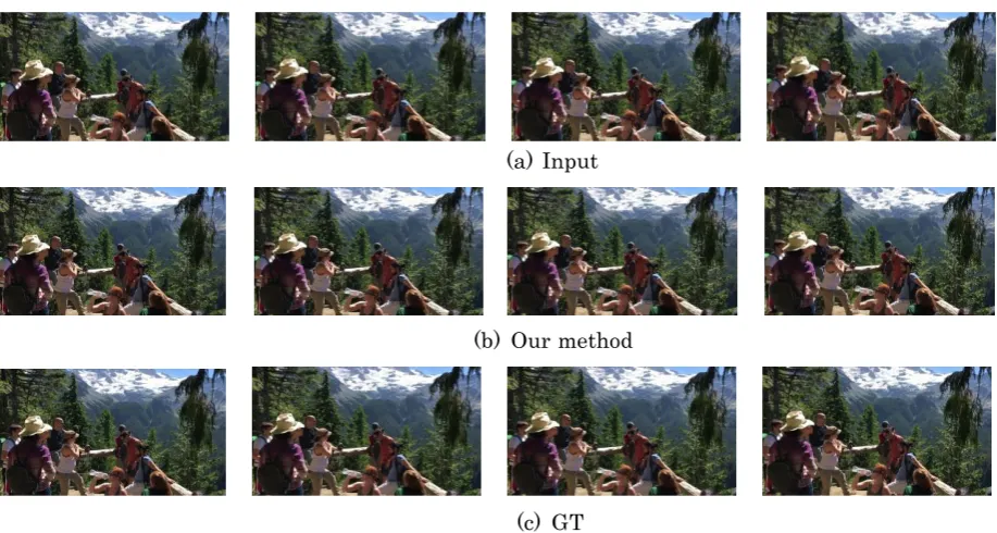
(a) Input

(b) Our method

(c) GT

Figure 5. (a) The first row shows the input frames from 96 to 99. (b) The second row shows the frames from 96 to 99 deblurred by our method. (c) The second row shows the GT(ground-truth) frames from 96 to 99.

Saliency Preserving Based Spatial Consistency Alignment

influences of spatially mesh-wise inconsistency in different regions. To this end, video re-targeting based on spatial structure consistency is utilized while preserving salient and visually prominent regions of each frame in the videos. Inspired by content-aware image and video retargeting techniques[4][17], to respect salient regions, we conduct homography estimation of spatial structure consistency.

Spatial Structure Consistency Optimization. A uniform grid is overlaid over the image with 𝑁^ columns and 𝑀^ rows. The target is to compute a deformed grid for the resized image. Consistent with common image retargeting methods, the saliency map 𝛹(𝑥^ , 𝑦^) is used to assign an importance value between 0 and 1 to every pixel of the image. A deformation that preserves the image in the salient zones as much as possible could be computed, and the unavoidable distortion could be concentrated in less important areas. We average the saliency values inside every cell of the grid on the original image, while the saliency vector 𝛹_𝑖 could be obtained.

Based on the saliency vector, our optimization makes further efforts to bring down the influences of spatially mesh-wise inconsistency, which greatly decrease the parallax. Using the method proposed by Lowe et al.[11], we could get the camera path and the local homographies. Then, we can define spatially mesh-wise inconsistent camera paths for the whole video. Let 𝐶_𝑖(𝑡) be the camera pose of the grid cell 𝑖 at frame 𝑡. It can be formulated as:

C_i(t) = C_i(t − 1)T_i(t − 1). (6) From Eq. (6, taking 𝐶𝑖(1) as the identity matrix, we can derive the next equation as:

Ci(t) = ∏t−1_t^=1Ti(t^). (7) We uniformly divide the frame into multiple grids. As shown in Fig. 4(b), 𝐷(𝑡) denotes the smoothed path, and 𝐵(𝑡) denotes the transformation from the original path 𝐶(𝑡) to the smoothed path 𝐷(𝑡).

As shown in Fig. 4(a), each grid has one trajectory, which is denoted by 𝐶_𝑖(𝑡). 𝑇_𝑖(𝑡 − 1) denotes the estimated local homographies at the same grid cell 𝑖 from 𝐶𝑖(𝑡 − 1) to 𝐶𝑖(𝑡). These camera trajectories of spatial structure consistency could be smoothed by

𝒪(D(t)) = argmin(Σ_i(‖D_i(t) − C_i(t)‖2_{+ λ}

tΨiΣj∈Ω(i)‖Di(t) − Dj(t)‖2)). (8) As shown in Eq. (8), 𝐶 = {𝐶(𝑡)} is the original path and 𝐷 = {𝐷(𝑡)} is the optimized path. 𝛺(𝑖) represents the eight neighbors of the grid cell 𝑖. Data term ‖𝐷_𝑖(𝑡) − 𝐶_𝑖(𝑡)‖ guarantees the new camera path to be close to the original one to reduce cropping and distortion, while ‖𝐷𝑖(𝑡) − 𝐷_𝑗(𝑡)‖ can keep the current grid cell be consistent with the nearby neighbors. Parameter 𝜆_𝑡 is used to balance the above two terms. For the marginal grid cell, we set its value is the same as those of its inexistent neighbors. Namely it can be formulated as 𝐷_𝑗(𝑡) = 𝐷_𝑖(𝑡) when 𝑗 is non-existent. This optimization is quadratic and its optimum result can be obtained by solving a large sparse linear system. The above solution is updated by a Jacobi-based iteration.

D_i(δ+1)= _1+2λC(t)

t+ Σ

2λtΨi

1+2λtDj

(δ)_.

(9)

In Eq. (9), 𝛿 is the iteration index. At initialization, 𝐷(0)(𝑡) = 𝐶(𝑡). Then we can get the optimized paths 𝐷𝑖(𝑡). Using 𝐵(𝑡) = 𝐶−1(𝑡)𝐷(𝑡), the original video frames could be transformed into the ones with spatial structure consistency while preserving salient regions.

Subsampling-convolution and Upsampling-convolution Module

We use a variation of Spatial Convolution and Spatial Full Convolution[20] for upsampling-convolutional and subsampling-convolution layers. As shown in second line of Fig. 1, 64@5,1 denotes 64 kernels in our convolution mode. Its kernel size is 5 × 5. Its stride is 1. 64@𝐻 × 𝑊 denotes the output size of our convolution model. 𝐻 denotes the height of the feature maps. 𝑊 denotes the weight of the feature maps. 64 denotes the number of feature maps. Other similar shapes mean something similar in the Fig. 1.

Subsampling-convolutional module consists of four pairs combination of flat-convolutional layer and the subsampling convolutional layer. The flat convolutional module is for non-linear mapping and preserve the size of the image. The subsampling layer can compress the spatial resolution of image features while increasing the spatial support of subsequent layers. During this process, many unclear areas are removed. During deep convolution of quadrilateral down sampling, most of the unsharp pixels are cleaned up. Upsampling-convolutional module consists of four pairs combination of flat-convolutional layer and the upsampling convolutional layer. The flat convolutional module is for non-linear mapping and preserve the size of the image. The upsampling convolutional layer could advance the spatial resolution while generating many new clear areas for the image. During this process, many clear areas are generated. During deep convolution of quadrilateral upsampling, most of the sharp pixels are successfully created.

(a) Input

(b) Delbracio et al. [3]

(c) Our method

Figure 6. (a) The first row shows the input four frames. (b) The second row shows the four frames deblurred by Delbracio et al.[3]. (c) The third row shows the four frames deblurred by our method.

Luckiness Threshold Value Based Back Propagation Module

This paper introduces a measurement of luckiness for a pixel in a video frame, which describes the absolute displacement of the pixel among adjacent frames. For a pixel p in frame 𝐷_𝑡, its luckiness is defined as

βt(p) = exp(−‖T˜t−1(p)−p‖

2_+‖T˜

t(p)−p‖2

2ϵ2 ). (10)

pixel position to another pixel position according to the homography T. 𝜖 is a constant which we empirically set as 20 pixels in our implementation. Eq. [equ.luckiness_measurement] computes the displacement of pixel p when the camera moves from frame 𝐷𝑡−1 to 𝐷𝑡+1 through 𝐷𝑡. When the frame-to-frame motion of p is small, 𝑇˜𝑡−1 and 𝑇˜𝑡 are close to 𝐼, thus 𝛽𝑡(𝑝) is close to 1, indicating that the image patch centered at p is likely to be sharp. Otherwise 𝛽𝑡(𝑝) is small, indicating that the patch is likely to contain large motion blur. The luckiness 𝛽_𝑡 of a whole frame 𝐷_𝑡 is simply defined as the average value of all 𝛽_𝑡(𝑝) for pixels in 𝐷_𝑡.

In the back propagation layer of our neural network, we introduce the luckiness measurement as the back propagation parameter. 𝔼(𝛽_𝑡) is the mathematical expectation value of all the frames. We empirically set 0.5 × 𝔼(𝛽_𝑡) as the luckiness threshold value. If the luckiness of the current frame is less than the luckiness threshold value, our deblurring process will go on. If not, we will get the sharp frame.

Experiments and Evaluations

Comparisons with State-of-The-Art Methods

Comparisons of frames deblurred by our method and GT. As shown in Fig. 5, the first row shows the input frames from 96 to 99. The second row shows the frames from 96 to 99 deblurred by our method. The third row shows the GT(ground-truth) frames from 96 to 99. The local region of the picture in the first row demonstrate that, the frame is seriously blurry. The local region of the picture in the second row demonstrate that, the frame is deblurred better. It can be seen from the contrast the local region of the picture in the second row with that in the third row, the pictures deblurred by our method are close to the ground-truth frames. The pictures and supplemented video could verify that, the video deblurred by our method is more unambiguous than the input video.

(a)Input

(b)Su et al. [20]

(c)Our method

Figure 7. (a) The first row shows the input frames from 96 to 99. (b) The second row shows the frames from 96 to 99 deblurred by Su et al.[20]. (c) The third row shows the frames from 96 to 99 deblurred by our method.

and supplemented video could verify that, the video deblurred by our method is more unambiguous than the video deblurred by Delbracio et al. [3].

Comparisons with Su et al.[20]. As shown in Fig. 7, the first row shows the input frames from 96 to 99. The second row shows the frames from 96 to 99 deblurred by Su et al.[20]. The third row shows the frames from 96 to 99 deblurred by our method. The local region of the picture in the first row demonstrate that, the frame is seriously blurry. The local region of the picture in the second row demonstrate that, the frame is deblurred to a certain degree. It can be seen from the contrast the local region of the picture in the second row with that in the third row, the pictures deblurred by our method are much clearer than those deblurred by Su et al. [20]. The pictures and supplemented video could verify that, the video deblurred by our method is more unambiguous than the video deblurred by Su et al. [20].

Comparisons of Frames Without Partial Module and Frames With All Modules

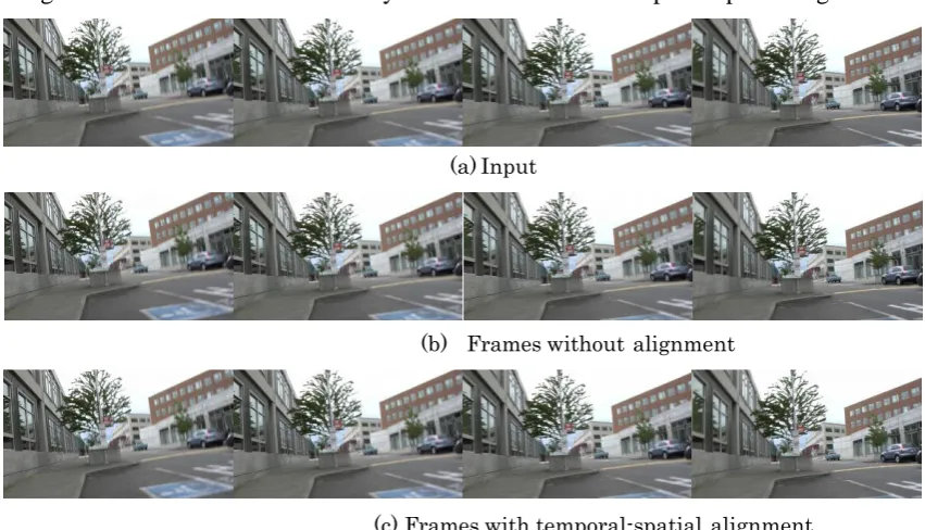
Comparisons of Frames without Alignment and Frames with Temporal-Spatial Alignment.

As shown in Fig. 8, the first row shows the input frames from 5 to 8. The second row shows the frames from 5 to 8 deblurred by our method without temporal-spatial alignment. The third row shows the frames from 5 to 8 deblurred by our method with temporal-spatial alignment. The local region of the picture in the first row demonstrate that, the frame is seriously blurry. The local region of the picture in the second row demonstrate that, the frame is deblurred to a certain degree. It can be seen from the contrast the local region of the picture in the second row with that in the third row, the pictures deblurred by our method with temporal-spatial alignment are much clearer than those deblurred by our method without temporal-spatial alignment. The pictures and supplemented video could verify that, the video deblurred by our method with temporal-spatial alignment is more unambiguous than the video deblurred by our method without temporal-spatial alignment.

(a)Input

(b) Frames without alignment

(c)Frames with temporal-spatial alignment

Figure 8. (a) The first row shows the input frames from 96 to 99. (b) The second row shows the frames from 96 to 99 deblurred by Su et al. [20]. (c) The third row shows the frames from 96 to 99 deblurred by our method.

Quantitative Evaluation

Conclusions and Discussions

In this paper, we have systematically presented a novel automatic method to address a suite of research challenges encountered in video deblurring. It is the first time that, the Neural Network improved via subsampling and upsampling is applied to the field of the video deblurring. With the help of space-time consistency alignment and luckiness threshold value based back propagation, our method could autonomously learn the optimization strategy for the video deblurring. The extensive experiments demonstrate the effectiveness of our method in handling wobbly videos with high-variability and broad-coverage of things and/or entities. All of these technical innovations contribute to automatic video deblurring with state-of-the-art performance in accuracy, versatility, flexibility, and efficiency. Nevertheless, our method may still have tremendous rooms to improve. For example, although our space-time consistency alignment based motion model could adaptively proceed the sharp pixels between the adjacent frames to deblur the video, however, it may bring about sacrificing accuracy of the result in some cases, such as severe occlusions and running. Besides, to minimize the geometrical distortion, our model tries our best efforts to enforce strong coherence between grid cells. In this way, it may further sacrifice image accuracy. The quality of the frames may be degraded while deblurring the unstable videos.

Acknowledgements

This research is supported in part by National Natural Science Foundation of China (NO. 61672077 and 61532002), Applied Basic Research Program of Qingdao (NO. 161013xx), National Science Foundation of USA (NO. IIS-0949467, IIS-1047715, IIS-1715985, and IIS-1049448), and capital health research and development of special 2016-1-4011.

Figure 9. Quantitative comparison of with other methods. In this plot, the PSNR[7] gain of applying different methods and confgurations is plotted versus the sharpness of the input frame. We observe that all methods provide a quality

improvement for blurry input frames, with diminishing improvements as the input frames get sharper.

References

[1] Aminnaji M, Aghagolzadeh A. Multi-Focus Image Fusion in DCT Domain using Variance and Energy of Laplacian and Correlation Coefficient for Visual Sensor Networks[J]. Journal of AI and Data Mining, 2018, 6(2): 233-250.

[2] Kuipers L, Timman R, Cohen J, et al. Handbook of mathematics[J]. The Mathematical Gazette, 1970, 54(389).

[4] Grundmann M, Kwatra V, Han M, et al. Discontinuous seam-carving for video retargeting[C]. computer vision and pattern recognition, 2010: 569-576.

[5] Iizuka S, Simoserra E, Ishikawa H, et al. Let there be color!: joint end-to-end learning of global and local image priors for automatic image colorization with simultaneous classification[J]. international conference on computer graphics and interactive techniques, 2016, 35(4).

[6] Joshi N, Cohen M F. Seeing Mt. Rainier: Lucky imaging for multi-image denoising, sharpening, and haze removal[C]. international conference on computational photography, 2010: 1-8.

[7] Kohler R, Hirsch M, Mohler B J, et al. Recording and playback of camera shake: benchmarking blind deconvolution with a real-world database[C]. european conference on computer vision, 2012: 27-40.

[8] Law N M, Mackay C D, Baldwin J E, et al. Lucky imaging: high angular resolution imaging in the visible from the ground[J]. Astronomy and Astrophysics, 2006, 446(2): 739-745.

[9] Lee K, Chuang Y, Chen B, et al. Video stabilization using robust feature trajectories[C]. international conference on computer vision, 2009: 1397-1404.

[10] Liu D, Wang Z, Wen B, et al. Robust Single Image Super-Resolution via Deep Networks With Sparse Prior[J]. IEEE Transactions on Image Processing, 2016, 25(7): 3194-3207.

[11] Lowe D G. Distinctive Image Features from Scale-Invariant Keypoints[J]. International Journal of Computer Vision, 2004, 60(2): 91-110.

[12] Matsushita Y, Ofek E, Ge W, et al. Full-frame video stabilization with motion inpainting[J]. IEEE Transactions on Pattern Analysis and Machine Intelligence, 2006, 28(7): 1150-1163.

[13] Michaeli T, Irani M. Blind Deblurring Using Internal Patch Recurrence[C]. european conference on computer vision, 2014: 783-798.

[14] Opower H. Multiple view geometry in computer vision: Richard Hartley, Andrew Zisserman, Cambridge University Press, Cambridge, 2000, 624 pages, Price £65.00, Hardback, ISBN 0-521-62304-9[J]. Optics and Lasers in Engineering, 2002, 37(1): 85-86.

[15] Park S H, Levoy M. Gyro-Based Multi-image Deconvolution for Removing Handshake Blur[C]. computer vision and pattern recognition, 2014: 3366-3373.

[16] Pathak D, Krahenbuhl P, Donahue J, et al. Context Encoders: Feature Learning by Inpainting[J]. computer vision and pattern recognition, 2016: 2536-2544.

[17] Rubinstein M, Shamir A, Avidan S, et al. Improved seam carving for video retargeting[J]. international conference on computer graphics and interactive techniques, 2008, 27(3).

[18] Sellent A, Rother C, Roth S, et al. Stereo Video Deblurring[J]. european conference on computer vision, 2016: 558-575.

[19] Shi W, Caballero J, Huszar F, et al. Real-Time Single Image and Video Super-Resolution Using an Efficient Sub-Pixel Convolutional Neural Network[J]. computer vision and pattern recognition, 2016: 1874-1883.

[20] Su S, Delbracio M, Wang J, et al. Deep Video Deblurring for Hand-Held Cameras[C]. computer vision and pattern recognition, 2017: 237-246.

[21] Su S, Heidrich W. Rolling shutter motion deblurring[C]. computer vision and pattern recognition, 2015: 1529-1537.

[23] Torr P H, Zisserman A. MLESAC: A New Robust Estimator with Application to Estimating Image Geometry[J]. Computer Vision and Image Understanding, 2000, 78(1): 138-156.

[24] Wang R, Tao D. Recent Progress in Image Deblurring[J]. arXiv: Computer Vision and Pattern Recognition, 2014.