The convergence analysis of P type iterative learning control with initial state error for some fractional system

R E S E A R C H

Open Access

The convergence analysis of P-type

iterative learning control with initial state

error for some fractional system

Xianghu Liu

_{and Yanfang Li}

*_{Correspondence:}

[email protected]

1_{Department of Mathematics,}

Guizhou University, Huaxi Road, Guiyang, China

2_{Mathematics Department, Zunyi}

Normal College, Wujiang Road, Zunyi, 563006, China

Abstract

In this paper, the convergence of iterative learning control with initial state error for some fractional equation is studied. According to the Laplace transform and the M-L function, the concept of mild solutions is showed. The sufficient conditions of convergence for the open and closed P-type iterative learning control are obtained. Some examples are given to illustrate our main results.

MSC: Primary 93C10; 93C40

Keywords: Caputo fractional derivative; iterative learning control; convergence; Mittag-Leffler function

1 Introduction

In this paper, we will analysis the convergence of iterative learning control initial state error of the following fractional system:

⎧ ⎪ ⎨ ⎪ ⎩

c_Dα

tx(t) =Ax(t) +Bu(t), t∈J= [,b], x() =x,

y(t) =Cx(t),

()

wherec_Dα

t denotes the Caputo fractional derivative of orderα,  <α< .A,B,C∈Rn×n, u(t) is a control vector.

Iterative learning control (ILC) was shown by Uchiyama in  (in Japanese), but only few people noticed it, Arimotoet al. developed the ILC idea and studied the effective algorithm until , they made it to be the iterative learning control theory, more and more people paid attention to it.

The fractional calculus and fractional difference equations have attracted lots of authors during in the past years, they published some outstanding work [–], because they de-scribed many phenomena in engineering, physics, science, and controllability. The work of fractional order systems in iterative learning control appeared in , and extensive attention has been paid to this field and great progress has been made in the following  years [–], many fractional nonlinear systems were researched [–]. To our knowl-edge, it has not been studied very extensively. In the study of iterative control theory, as-sume that the initial state of each run is on the desired trajectory, however, the actual

operation often causes some error from the iterative initial state to the desired trajectory, so we consider the system () and study the convergence of the learning law.

Motivated by the above mentioned works, the rest of this paper is organized as follows: In Section , we will show some definitions and preliminaries which will be used in the following parts. In Sections  and , we give some results for P-type ILC for some fractional system. In Section , some simulation examples are given to illustrate our main results.

In this paper, the norm for then-dimensional vectorw= (w,w, . . . ,wn) is defined as w=max≤i≤n|wi|, and theλ-norm is defined asxλ=sup_t∈[,T]{e–λt|x(t)|},λ> .

2 Some preliminaries for some fractional system

In this section, we will give some definitions and preliminaries which will be used in the paper, for more information, one can see [–].

Definition . The integral

Iα

tf(t) =  (α)

t 

(t–s)α–_{f(s)ds, α> ,}

is called the Riemann-Liouville fractional integral of orderα, whereis the gamma func-tion.

For a functionf(t) given in the interval [,∞), the expression

L_Dα

tf(t) =  (n–α)

d dt

n t 

(t–s)n–α–f(s)dt,

wheren= [α] + , [α] denotes the integer part of numberα, is called the Riemann-Liouville fractional derivative of orderα> .

Definition . Caputo’s derivative for a functionf : [,∞)→Rcan be written as

c_Dα

tf(t) =LD

α

t f(t) – n–

k= tk k!f

(k)_()

, n= [α] + ,

where [α] denotes the integer part of real numberα.

Definition . The definition of the two-parameter function of the Mittag-Leffler type is described by

Eα,β(z) =

∞

k= zk

(αk+β), α> ,β> ,z∈C,

ifβ= , we get the Mittag-Leffler function of one parameter,

Eα(z) =

∞

k= zk (αk+ ).

Lemma . The general solution of equation()is given by

x(t) =Sα,(A,t)x+

t 

Sα,α(A,t–s)Bu(s)ds, ()

Sα,β(A,t) =

∞

k=

Ak_tαk+β– (αk+β).

Lemma . From Definition.in[],we know that the operators Sα,(t),Sα,α(t),Sα,α–(t) are exponentially bounded,there is a constant C=_α,C=_αA

–α α ,C_=

αA

–α α ,e_α(t) =

eA

 αt_,M=e

α(b),

Sα,(A,t)≤Ceα(t), Sα,α(A,t)≤Ceα(t). ()

3 Open and closed-loop case

In this section, we consider the following fractional equation:k= , , , , . . . ,

c_Dα

txk(t) =Axk(t) +Buk(t), t∈J= [,b], yk(t) =Cxk(t).

()

For equation (), we apply the following open and closed-loop P-type ILC algorithm, t∈[,b]:

uk+(t) =uk(t) +Lek(t) +Lek+(t), ()

whereL,Lare the parameters which will be determined,ek=yd(t) –yk(t),yd(t) are the given functions. The initial state of each iterative learning is

xk+() =xk() +BLek(t). ()

We make the following assumptions:

(H):  –λ–CMCLB> ,

(H): I–CSα,(A,t)BL+λ–CMCLB –λ–_C

MCLB < .

Theorem . Assume that the open and closed-loop P-type ILC algorithm()is used, (H) and(H)hold,let yk(·)be the output of equation(),if the initial state of each iterative learning satisfy(),lim_k→∞ekλ= ,t∈J.

Proof According to (), (), and (), we know

xk+(t) =Sα,(A,t)xk+() +

t 

Sα,α(A,t–s)Buk+(s)ds

=Sα,(A,t)

xk() +BLek(t)

+

t 

Sα,α(A,t–s)B

uk(s) +Lek(s) +Lek+(s)

ds

=xk(t) +Sα,(A,t)BLek(t) +

t 

Sα,α(A,t–s)BLek(s)ds

+

t 

so the (k+ )th iterative error is

ek+(t) =yd(t) –Cxk+(t)

=yd(t) –C

xk(t) +Sα,(A,t)BLek(t) +

t 

Sα,α(A,t–s)BLek(s)ds

+

t 

Sα,α(A,t–s)BLek+(s)ds

=ek(t) –C

Sα,(A,t)BLek(t) +

t 

Sα,α(A,t–s)BLek(s)ds

+

t 

Sα,α(A,t–s)BLek+(s)ds

=I–CSα,(A,t)BL

ek(t) –C

t 

Sα,α(A,t–s)BLek(s)ds

–C

t 

Sα,α(A,t–s)BLek+(s)ds; ()

take the norm of (),

ek+(t)≤I–CSα,(A,t)BLek(t)

+C

t 

Ceα(s)BLek(s)ds

+C

t 

Ceα(s)BLek+(s)ds, ()

take theλ-norm of (),

ek+λ≤I–CSα,(A,t)BLekλ

+ sup

t∈[,T]e –λt_CC

BL

t 

_eα(s)ek(s)ds

+ sup

t∈[,T]e –λt_C

t 

Ceα(s)BLek+(s)ds

≤I–CSα,(A,t)BLekλ

+ sup

t∈[,T]e –λt_CC

BL

t 

eα(s)eλsdsekλ

+ sup

t∈[,T]e –λt_C

t 

Ceα(s)BLeλsdsek+λ, ()

if  –λ–_C

MCLB> ,

ek+λ≤

I–CSα,(A,t)BL+λ–CMCLB  –λ–_C

MCLB

ekλ, ()

let I–CSα,(A,t)BL+λ–CLMCB

Theorem . implied that the tracking errorek(t) depends onCandxk(t), it is also ob-served for () that the boundedness of the parametersC,B,L,Limplies the bounded-ness of theekλ, so Theorem . indirectly indicated that the output error also depend

on I–CSα,(A,t)BL+λ–CMCLB

–λ–CMCLB . From the result, we can do a more in-depth discussion.

Corollary . Suppose that all conditions are the same with Theorem.,lim_k→∞ekλ=

,then

lnCML+CML

λCL Aα

<t<b.

Proof From Theorem ., the important condition is I–CSα,(A,t)BL+λ–CMCLB –λ–_C

MCLB < , which implies that

 –Ceα(t)CLB+λ–CMCLB ≤ –λ–CMCLB,

we can get

lnCML+CML

λCL Aα

<t<b.

4 P-type ILC for some fractional system with random disturbance

In this section, we consider the following fractional equation:k= , , , , . . . ,

c_Dα

txk(t) =Axk(t) +Buk(t) +ωk(t), t∈J= [,b], yk(t) =Cxk(t) +νk(t),

()

whereωk(t),νk(t) are the random disturbance.

Firstly, we will make some assumptions to be satisfied on the data of our problem:

(H): ωkλ≤ε,νkλ≤εfor some positive constantsε,ε,

(H): ρ=I+CSα,(A,t)LB–λ–CCLBM> , ρ=I–CSα,(A,t)LB+λ–CCLBM.

For equation (), we choose the following open and closed-loop P-type ILC algorithm, t∈[,b]:

uk+(t) =uk(t) +Lek(t) +Lek+(t), ()

whereL,Lare the parameters which will be determined,ek=yd(t) –yk(t),yd(t) are the given functions.

Assume that the initial state of each iterative learning is (), whereL,Lare the pa-rameters which will be determined. We have

xk+() =xk() +BLek(t) +BLek+(t). ()

Proof According to () and assumptions (H), (H), we know

xk+(t) =Sα,(A,t)xk+() +

t 

Sα,α(A,t–s)

Buk+(s) +ωk+(s)

ds

=Sα,(A,t)

xk() +BLek(t) +BLek+(t)

+

t 

Sα,α(A,t–s)B

uk(s) +Lek(s) +Lek+(s)

ds

+

t 

Sα,α(A,t–s)ωk+(s)ds

=xk(t) +Sα,(A,t)BLek(t) +Sα,(A,t)BLek+(t)

+

t 

Sα,α(A,t–s)BLek(s)ds+

t 

Sα,α(A,t–s)BLek+(s)ds

+

t 

Sα,α(A,t–s)ωk+(s)ds,

the (k+ )th iterative error is

ek+(t) =yd(t) –Cxk+(t) –νk+(t)

=yd(t) –C

xk(t) +Sα,(A,t)BLek(t) +Sα,(A,t)BLek+(t)

+

t 

Sα,α(A,t–s)BLek(s)ds+

t 

Sα,α(A,t–s)BLek+(s)ds

+

t 

Sα,α(A,t–s)ωk+(s)ds

–νk+(t)

=ek(t) –C

Sα,(A,t)BLek(t) +Sα,(A,t)BLek+(t)

+

t 

Sα,α(A,t–s)BLek(s)ds+

t 

Sα,α(A,t–s)BLek+(s)ds

+

t 

Sα,α(A,t–s)ωk+(s)ds

–νk+(t)

=I–CSα,(A,t)BL

ek(t) –CSα,(A,t)BLek+(t)

–C

t 

Sα,α(A,t–s)BLek(s)ds–C

t 

Sα,α(A,t–s)BLek+(s)ds

–C

t 

Sα,α(A,t–s)ωk+(s)ds–νk+(t). ()

Taking the norm of (), it is easy to obtain

I+CSα,(A,t)LBek+(t)

≤I–CSα,(A,t)LBek(t)+C

t 

Ceα(s)LBek(s)ds

+C

t 

Ceα(s)LBek+(s)ds+C

t 

Ceα(s)ωk+(s)ds

once more using theλ-norm, we have

I+CSα,(A,t)LBek+λ

≤I–CSα,(A,t)LBekλ+ sup

t∈[,T]e –λt_C

CBL

t 

_eα(s)eλsdsekλ

+ sup

t∈[,T]e –λt_C

CLB

t 

eα(s)eλsdsek+λ

+ sup

t∈[,T]e –λt_C

C

t 

eα(s)eλsdsωk+λ+ sup

t∈[,T]e –λt_ν

k+(t),

invoking (H) and (H), ifε=λ–CεMC+ε,

ρek+λ≤ρekλ+ε, ()

which implies that

ekλ≤

ε ρ–ρ

,

ifε→ andε→,ε→, thuslimk→∞ekλ= ,t∈J, and this completes the proof.

From Theorem ., on the one hand, the random disturbance makes some impact on the system (),ε→ andε→ imply the impact is very small; on the other hand,ρ>ρ, for this condition, we illustrate the following corollary.

Corollary . Suppose that all conditions are the same as Theorem.,lim_k→∞ek(t)λ=

,then t satisfies

ln|CM

λC| Aα

<t<ln|

–λ–CCLBM CLB | Aα

.

Proof According to (H),I+CSα,(A,t)LB–λ–CCLBM> , then

t<ln|

–λ–CCLBM CLB | Aα

.

From Theorem ., we know thatε→ andε→, and the condition is

ρ ρ

=I–CSα,(A,t)LB+λ –_C

CLBM I+CSα,(A,t)LB–λ–CCLBM

< ,

which yields ln|

C_M

λC|

Aα <t. At last, we obtain the estimate

ln|CM

λC| Aα

<t<ln|

–λ–CCLBM CLB | Aα

5 Simulations

In this section, we will give two simulation examples to demonstrate the validity of the algorithms.

5.1 P-type ILC with initial state error

⎧ ⎪ ⎨ ⎪ ⎩

c_D.

t xk(t) =xk(t) + .uk(t), t∈J= [, .], x() = .,

yk(t) =xk(t),

()

with the iterative learning control and initial state error

uk+(t) =uk(t) + .ek(t) + .ek+(t), xk+() =xk() + .ek(t).

()

We set the initial controlu(·) = ,yd(t) = t( – t),t∈(, .), and setα= .,A= , B= .,C= .,λ= ,L=L= ., andC= ,C= ,λ–A



α _{=  > ,M}≈_{ > ,}

 –λ–_C

MCLB ≈. > , I–CSα,(A,t)BL+λ –_C

MCLB –λ–_C

MCLB ≈ .

. < , all conditions of Theorem . are satisfied.

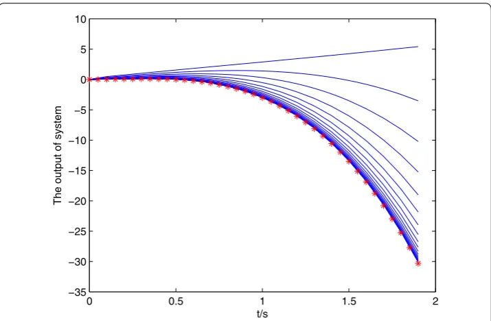
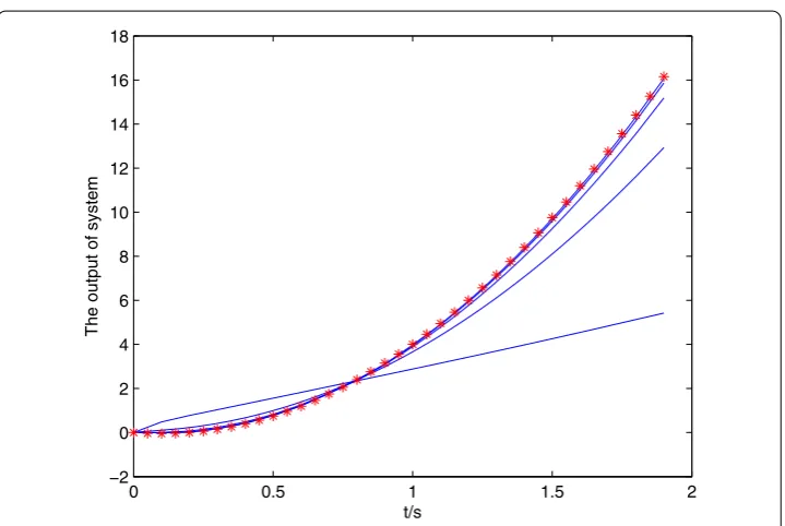
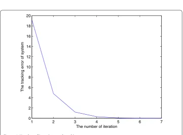
The simulation result can be seen from Figure  and Figure , for the open and closed-loop P-type ILC system (), with the increase of the number of iterations, it can track the desired trajectory gradually by using the algorithm. We do not use the single iteration rate to get the result, because in the late of the iteration, the output of the system may jump around the desired trajectory, so we adopt a correction method, that is, whene(k) > , u(k) =u(k) – .×e(k) ore(k) < ,u(k) =u(k) + .×e(k),kis the number of iteration, the result approaches the desired trajectory stably and quickly, from Figure , the tracking error tends to zero at the th iteration, so the iterative learning control is feasible and the efficiency is high.

Figure 2 Number of iterations and tracking error.

5.2 P-type ILC with random disturbance

Consider the following P-type ILC system:

⎧ ⎪ ⎨ ⎪ ⎩

c_D.

t xk(t) =xk(t) + .uk(t) + –t, t∈J= [, .], x() = .,

yk(t) = .xk(t) + –t,

()

with the iterative learning control and initial state error

uk+(t) =uk(t) +ek(t) + .ek+(t), xk+() =xk() + .ek(t) + .ek+(t).

()

We set the initial controlu(·) = ,yd(t) = t–t,t∈(, .), and setα= .,A= , B= .,C= ,λ= ,L= ,L= ., andC= ,C= ,ρ≈.,ρ≈.,ε= –→ ,ε= –→, all conditions of Theorem . are satisfied. We also use a correction method, that is, whene(k) > ,u(k) =u(k) –m×e(k) ore(k) < ,u(k) =u(k) +m×e(k), k is the number of iterations, m is the parameter, we set m= ., ., , and the out-put of the system is shown in Figure , Figure , Figure . The symbol∗∗∗denotes the desired trajectory, — denotes the output of the system, the tracking error is shown in Figure , Figure , Figure , which imply the number of iteration and the tracking er-ror.

Figure 3 ∗∗∗denotes the desired trajectory, — denotes the output of the system.

Figure 5 ∗∗∗denotes the desired trajectory, — denotes the output of the system.

Figure 7 Number of iterations and tracking error.

Figure 8 Number of iterations and tracking error.

Table 1 The iteration number and the tracking error and the running time table

m The number of iterations The tracking error Run time (second)

0.5 7 0.002 58.207

0.7 5 0.0013 50.123

Competing interests

The authors declare that they have no competing interests.

Authors’ contributions

The authors contributed equally to this work. All authors read and approved the final manuscript.

Acknowledgements

This work was financially supported by the Zunyi Normal College Doctoral Scientific Research Fund BS[2014]19, BS[2015]09, Guizhou Province Mutual Fund LH[2015]7002, Guizhou Province Department of Education Fund KY [2015]391, [2016]046, Guizhou Province Department of Education teaching reform project [2015]337, Guizhou Province Science and technology fund (qian ke he ji chu) [2016]1160, [2016]1161, Zunyi Science and technology talents [2016]15.

Received: 15 September 2016 Accepted: 19 January 2017

References

1. Miller, KS, Ross, B: An Introduction to the Fractional Calculus and Differential Equations. Wiley, New York (1993) 2. Kilbas, AA, Srivastava, HM, Trujillo, JJ: Theory and Applications of Fractional Differential Equations. Elsevier,

Amsterdam (2006)

3. Lakshmikantham, V, Leela, S, Devi, JV: Theory of Fractional Dynamic Systems. Cambridge Academic Publishers, Cambridge (2009)

4. Diethelm, K: The Analysis of Fractional Differential Equations. Springer, Berlin (2010)

5. Wang, JR, Zhou, Y, Medved, M: On the solvability and optimal controls of fractional integrodifferential evolution systems with infinite delay. J. Optim. Theory Appl.152, 31-50 (2012)

6. Zhang, L, Ahmad, B, Wang, G: Explicit iterations and extremal solutions for fractional differential equations with nonlinear integral boundary conditions. Appl. Math. Comput.268, 388-392 (2015)

7. Zhang, X: On the concept of general solution for impulsive differential equations of fractional-orderq∈(1, 2). Appl. Math. Comput.268, 103-120 (2015)

8. Ge, F-D, Zhou, H-C, Ko, C-H: Approximate controllability of semilinear evolution equations of fractional order with nonlocal and impulsive conditions via an approximating technique. Appl. Math. Comput.275, 107-120 (2016) 9. Arthi, G, Park, JH, Jung, HY: Existence and exponential stability for neutral stochastic integrodifferential equations with

impulses driven by a fractional Brownian motion. Commun. Nonlinear Sci. Numer. Simul.32, 145-157 (2016) 10. Hernández, E, O’Regan, D, Balachandran, K: On recent developments in the theory of abstract differential equations

with fractional derivatives. Nonlinear Anal.73, 3462-3471 (2010)

11. Zayed, EME, Amer, YA, Shohib, RMA: The fractional complex transformation for nonlinear fractional partial differential equations in the mathematical physics. J. Assoc. Arab Univ. Basic Appl. Sci.19, 59-69 (2016)

12. Zhang, X, Zhang, B, Repovš, D: Existence and symmetry of solutions for critical fractional Schrödinger equations with bounded potentials. Nonlinear Anal., Real World Appl.142, 48-68 (2016)

13. Bien, Z, Xu, JX: Iterative Learning Control Analysis: Design, Integration and Applications. Springer, New York (1998) 14. Chen, YQ, Wen, C: Iterative Learning Control: Convergence, Robustness and Applications. Springer, Berlin (1999) 15. Norrlof, M: Iterative Learning Control: Analysis, Design, and Experiments. Linkoping Studies in Science and

Technology, Dissertations, Sweden (2000)

16. Xu, JX, Tan, Y: Linear and Nonlinear Iterative Learning Control. Springer, Berlin (2003)

17. Wang, Y, Gao, F, Doyle III, FJ: Survey on iterative learning control, repetitive control, and run-to-run control. J. Process Control19, 1589-1600 (2009)

18. de Wijdeven, JV, Donkers, T, Bosgra, O: Iterative learning control for uncertain systems: robust monotonic convergence analysis. Automatica45, 2383-2391 (2009)

19. Xu, JX: A survey on iterative learning control for nonlinear systems. Int. J. Control84, 1275-1294 (2011)

20. Li, Y, Chen, YQ, Ahn, HS: Fractional-order iterative learning control for fractional-order systems. Asian J. Control13, 54-63 (2011)

21. Lan, Y-H: Iterative learning control with initial state learning for fractional order nonlinear systems. Comput. Math. Appl.64, 3210-3216 (2012)

22. Lin, M-T, Yen, C-L, Tsai, M-S, Yau, H-T: Application of robust iterative learning algorithm in motion control system. Mechatronics23, 530-540 (2013)

23. Yan, L, Wei, J: Fractional order nonlinear systems with delay in iterative learning control. Appl. Math. Comput.257, 546-552 (2015)

24. Liu, S, Wang, JR, Wei, W: Analysis of iterative learning control for a class of fractional differential equations. J. Appl. Math. Comput.53, 17-31 (2017)

25. Liu, S, Debbouche, A, Wang, J: On the iterative learning control for stochastic impulsive differential equations with randomly varying trial lengths. J. Comput. Appl. Math.312, 47-57 (2017)

26. Zhou, Y, Jiao, F: Existence of mild solutions for fractional neutral evolution equations. Comput. Math. Appl.59, 1063-1077 (2010)

27. Mophou, GM, N’Guérékata, GM: Existence of mild solutions of some semilinear neutral fractional functional evolution equations with infinite delay. Appl. Math. Comput.216, 61-69 (2010)

28. Wei, J: The controllability of fractional control systems with control delay. Comput. Math. Appl.64, 3153-3159 (2012) 29. Yan, L, Wei, J: Fractional order nonlinear systems with delay in iterative learning control. Appl. Math. Comput.257,

546-552 (2015)