2019 International Conference on Computer Intelligent Systems and Network Remote Control (CISNRC 2019) ISBN: 978-1-60595-651-0
CT Image Segmentation of Liver Tumor Based on
Improved Convolution Neural Network
Qinglu Jiao, Zhifei Li and Shuni Song
ABSTRACT
In this paper, an improved cross entropy loss function CNN structure is proposed to segment images, and a group of original three-phase images of liver tumors are input into the network for training. Finally, the dice coefficient (DSC) of the segmentation results of this method is 96%, the accuracy is 86% and the recall rate is 89%.The results show that the improved cross entropy loss function CNN structure is more conducive to the segmentation of liver tumors, with a higher accuracy. Meanwhile, it is proved that the algorithm converges when the correlation conditions are satisfied.
KEYWORDS
Image segmentation, Convolution neural network, Loss function, three-phase CT image.
INTRODUCTION
The liver plays an important role in urea synthesis and metabolism in human beings, but the liver is also one of the most common sites of tumor and the resection is the main method for the treatment of liver tumors. The segmentation result of liver tumor image is an important basis for resection is the main method for the treatment of liver tumors resection. With the rapid development of computer technology, the computer aided diagnosis technology based on medical imaging has made rapid development. It separates the suspected lesions from the normal anatomical background, so as to help doctors improve the work efficiency and the accuracy of diagnosis. Today CT image has been widely used in radiology department because of its high resolution and reasonable charge pricing. Therefore, how to use modern information technology to segment CT images of liver tumors efficiently and automatically has become an important research direction.
With the further development of research work, CT image segmentation gradually changes from two-dimensional to three-dimensional research, and the loss function for neural network is also gradually improved. In 2016, Li Wen[1] proposed a CT image liver tumor segmentation method based on deep convolution neural network, and the logarithm likelihood function is used as the loss function. Compared with the traditional machine learning algorithm, the image ________________________________________
features of convolution neural network autonomous learning are more effective and divisible, which is beneficial to tumor segmentation. In same year, Ben-Cohen[2] proposed a Fully Convolution Network segmentation method for CT image liver tumor segmentation, Peijun Hu[3] proposed an automatic segmentation framework based on three-dimensional convolution neural network and global optimization surface evolution. The logarithm likelihood function is also used in it. In 2017, Eli Gibson[4] defined a CNN architecture comprising fully-convolutional deep residual networks with multi-resolution loss function. However, there exists sample imbalance in liver tumor images, and the cross-entropy loss function has some defects in dealing with sample imbalance. In 2018, Kai Hu[5] proposed an improved cross entropy loss function for retinal vascular segmentation of color fundus images. The recall rate increased from 75.23% to 75.52%, which indicates that the improved cross entropy loss function is suitable for unbalanced retinal vessels. Fu, YB[6] proposed a depth learning model for automatic segmentation of liver, kidney, stomach, intestine and duodenum in three-dimensional MR images. The model includes a voxel direction label prediction CNN and a correction network composed of two subnetworks.
At the same time, the study of CT images of liver tumors is also transferring from single phase data to multi-phase data, which can extract and utilize three-dimensional information as much as possible. Ji Zhiyuan[7] proposed a classification problem of liver tumors based on multi-phase three-dimensional CT images. Peng Gu[8] designed an 8-layer convolution neural network combined with a neural network for comprehensive evaluation to segment three-dimensional breast ultrasound images into four main tissues: skin, fibrogland tissue, mass and adipose tissue, and achieved good segmentation results. The above provides a new idea for our research.
DATAPREPARATION
BACKGROUNDKNOWLEDGEOFCTIMAGESOFLIVERTUMORS
[image:2.595.197.396.620.688.2]The plain scanning phase refers to the period without contrast agent injection, the arterial phase(ART) is within 30-40 seconds after contrast agent injection, the portal vein phase(PV) is within 70-80 seconds after contrast agent injection, and the delayed phase(DL) is 3-5 minutes after contrast agent injection. CT images of typical liver tumors in phase iii of ART, PV and DL are shown in Figure 1:
DATAACQUISITION
[image:3.595.112.474.193.271.2]The liver CT image data in this paper are from The Cancer Genome Atlas Program (TCGA)[10] .This joint effort between the National Cancer Institute and the National Human Genome Research Institute began in 2006, bringing together researchers from diverse disciplines and multiple institutions. In this paper, the CT images of liver tumors in this database (TCGA-LIHC) are selected as samples for training in the network.
[image:3.595.137.449.344.450.2]Figure 2. CT image training sample of liver tumor.
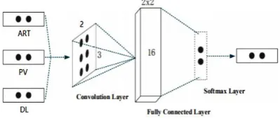
Figure 3. Convolution Neural Network structure of Pixel Classification.
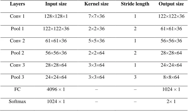
TABLE I. CNN STRUCTURE PARAMETER TABLE FOR PIXEL CLASSIFICATION.
Layers Input size Kernel size Stride length Output size
Conv 1 128×128×1 7×7×36 1 122×122×36
Pool 1 122×122×36 2×2×36 2 61×61×36
Conv 2 61×61×36 5×5×36 1 56×56×36
Pool 2 56×56×36 2×2×64 2 28×28×64
Conv 3 28×28×64 3×3×64 1 24×24×64
Pool 3 24×24×64 3×3×64 3 8×8×64
FC 4096 × 1 – – 1024 × 1
[image:3.595.106.472.559.778.2]DATAPROCESSING
The downloaded image is Dicom file type. The picture sample is read by Python to convert the original gray image into a meaningful array of CNNs numbers. Create true tags and store them as segmented tags for training input images. The image block is divided into training set and test set, and the pixels in the training set image block are marked according to the true value label, which is used for network training. The segmentation effect is evaluated by using the test set.
METHOD
In this paper, the neural network architecture adopts the network structure of double network in reference[8] to process the third phase image data of liver tumor CT image.
NETWORK DESIGN
The original three phase image data are used as input, and an 8-layer CNN (CNN-I) is used for network training. The region of interest (ROI) of tumor data is obtained from the original image and label information according to the original image and label information. The CNN schema and detailed configuration parameters are shown in Table II and Figure 3. The input image size is selected as 128*128 through the pre-experiment.
After the forward propagation of the network, the original data is output to the probability value of tumor or non-tumor by sigmoid classification function, and the two probability values of the output array indicate the probability tags of tumor and non-tumor. The index of the maximum element determines the central pixel in the image block. The size and layer number of each core were determined in the pre-experiment. In order to capture the nonlinear mapping between input and output, all convolution layers and fully connected layers are activated by sigmoid function.
Figure 4. CNN Structure for Comprehensive Classification.
THE IMPROVED CROSS-ENTROPY LOSS FUNCTION
The cross entropy loss function can not only simplify the computation of the network, but also effectively overcome the problem of slow convergence of the sigmoid function. Because there are a lot of interference terms in CT images of liver tumors, if the loss function does not consider the problem of sample balance, the learning process will tend to segment most of the non-tumor tissues. Therefore, we use the class equilibrium cross entropy loss function to improve the original loss function as follows.
))] ( 1 log( ) 1 ( ) ( log [
) ,
( j
Y j
j y
y b
L
where Y and Y represent tumor and non-tumor pixels, respectively. The weights β and α are used for the balance class, and β is represented by the ratio of tumor pixels to all pixels. α is a superparameter and we set it to 2.5 in the experiment. (yj) represents the probability that the sigmoid function is active at pixel j.
PROOF OF CONVERGENCE OF FULL CONNECTION LAYER OF NEURAL NETWORK
Assuming that the number of neural units in the input layer and the hidden layer is Q,P. The essence of liver tumor image segmentation is the binary
classification of image pixels, so the number of neurons in the output layer is 2.
The training sample set is recorded as
T j j j Q
J j j j
o o O R R
O} ( , )
,
{ 2 1 2
1
,
, where 2
, 1 ), 1 , 0
(
t
otj . The weight matrix between the output layer and the hidden layer
is recorded as V(Vpq)PQ , where v (v1,v 2,...,v ) R ,p 1,2,...,P.
Q T pQ p p
p The
connection right matrix between the hidden layer and the output layer is denoted
as W (wtp)2P , where w (w1,w2,...,w ) R ,t1,2
P T tp t t
t . Set g:RP as
nonlinear smooth activation function of each node in hidden layer,
R x e
x x
,
1 1 ) (
is activation function for each node in the output layer.
After the sample
Q j
R
is input into the network, the actual output of the
network is
. ,... 2 , 1 , 2 , 1 )), (
(w GV t j J
f j
t j
t
n n
V
W , denote the weight matrix after the training of the nth cycle in the network training.
n
denotes the learning rate of the nth training. n varies according to the
following rules: For an arbitrary initial value 00,
1
1 1
n n
n1,2,...,
When the improved cross entropy loss function is used in the process of network training, we have
J
j t
j t j
t GV f w GV
w f V
W E
1 2
1
)))] ( ( 1 ln( ) 1 ( ))) ( ( ln( [ ) ,
(
The gradient function of the weight matrix W,V corresponding to the fully
connected layer is
J
j t
j j p tp j t j
t v
J
j t
j j
t j
t w
v g w V
G w f V
G w f V
W E
V G V
G w f V
G w f V
W E
p t
1 2
1 1
2
1
) ( ) )) ( ( ) 1 ( )) ( ( ( ) , (
) ( ) )) ( ( ) 1 ( )) ( ( ( ) , (
When existing an C10 satisfied the following conditions:
R x k
C x
gk( )| , 0,1,2 |
) 1
( 1
) (
2 , 1 1
2 , 1 , 0 , | ) ( | ) 2
( h(k) x C1 k xR jJ t
jt
where
P p
p p
jt x O f x O f x
h
1
))] ( 1 ln( ) 1 ( ) ( ln [ )
(
,... 2 , 1 , 1 , || || ,...; 2 , 1 , 2 , 1 , || || ) 3
( w C1 t n v C pPn n
p n
i
the fully connection layer weight matrix of convolution neural networks is converged[11].
For any given initial weight matrics W MTP 0
,V0MPQ, {Wn,Vn}is generated
by a reverse propagation algorithm based on improved cross-entropy function
criterion. Then when the learning rate
new n
is little enough, there exists N00, which let every nN has
) , ( )
(Wn1 Vn 1 EWn Vn
And There also exists *0
E , so that *
) , (
limEWnVn E
n
can be established.
Proof For any t1,2,j1,2,...,J and n1,2,..., we have
2 1 1 , , 1 1 1 1 )] ( ) ( )))[ ( 1 )( ( ( 2 1 )] ( ) ( )[ 1 )) ( ( ( )) ( ( ln )) ( ( ln j n n t j n n t j t j t j n n t j n n t j n n t j n n j n n t V G w V G w u f u f V G w V G w V G w f V G w f V G w f t 2 1 1 , , 1 1 1 1 )] ( ) ( )))[ ( 1 )( ( ( 2 1 )] ( ) ( )))[ ( ( ( ))] ( ( 1 ln[ ))] ( ( 1 ln[ j n n t j n n t j t j t j n n t j n n t j n n t j n n j n n t V G w V G w v f v f V G w V G w V G w f V G w f V G w f t
where ( ) (1 , ) ( ), , (0,1)
1 1 , , j t j n n t j t j n n t j t j
t w GV w GV
u
) 1 , 0 ( ), ( ) 1 ( ) ( , , 1 1 , , j t j n n t j t j n n t j t j
t w GV w GV
v
We can also get the conclusion in the same way that
2 ,
1 ''( )( )
2 1 ) )( ( ' ) ( )
( n j
p j p j n p j n p j n p j n
p gv g v v g l v
v
g
where ( 1 (1 ) ) , (0,1), 1,2,... .
, v v p P
l p j n p p n p p j
p
Then P p j n p j p j n p j n p n tp P p j n p j n p n pt j n j n n t v l g v v g w v g v g w V G V G w 1 2 , 1 1 1 ) ) )( ( '' 2 1 ) )( ( ' ( )) ( ) ( ( )) ( ) ( ( And P p J j t P p t n p j p n tp j n n t n p new n J j t j n j n n t j t j n n t v l g w V G w f v V G V G w O V G w f 1 1 2 1 1 2 , 2 1 2 1 1 ) )( ( '' ) )) ( ( ( 2 1 || || 1 )) ( ) ( ( ) )) ( ( (
For any t1,2,j1,2,...,J and n1,2,...,
) ( )) ( ) ( ( )) ( ) ( ( ) ( ) ( 1 1 1 1 j n n t j n j n n t j n j n n t j n n t j n n t V G w V G V G w V G V G w V G w V G w
} )] ( ) ( ))[ ( 1 )( ( 2 ) 1 ( )] ( ) ( ))[ ( 1 )( ( 2 )] ( ) ( )[ 1 )) ( ( ( ) 1 ( )] ( ) ( )[ )) ( ( ( { ] )) ( 1 ( ln ) 1 ( )) ( ( ln [ ))] ( 1 ( ln ) 1 ( )) ( ( ln [ ) , ( ) , ( 2 1 1 , 2 1 1 , , 1 1 1 2 1 1 1 1 2 1 1 2 1 1 1 1 1 1 1 j n n t j n n t j t j t j n n t j n n t j t j t j n n t j n n t j n n t J j t j n n t j n n t j n n t J j t j n n j n n J j t j n n j n n n n n n V G w V G w v f v f V G w V G w u f u f V G w V G w V G w f V G w V G w V G w f V G w f V G w f V G w f V G w f V W E V W E
Where is a constant that greater than 1, so 10, and 01,
1 )) ( (
0 n n j t GV
w
f ,
then 0 ) 1 )) ( ( ( ) 1
( f wtnGVnj
So for any j1,2,...,J
if 1 ( 1 ) n ( n j)0
t j n n
t GV w GV
w ,then
)] ( )[ )) ( ( ( )] ( ) ( )[ 1 )) ( ( ( ) 1 ( )] ( )[ )) ( ( ( 1 1 1 1 1 1 j n n t j n n t j n n t j n n t j n n t j n n t j n n t V G w V G w f V G w V G w V G w f V G w V G w f
if 1 ( 1 ) n ( n j)0
t j n n
t GV w GV
w ,then
)] ( )[ )) ( ( ( )] ( ) ( )))[ ( ( )( 1 )( 1 ( )] ( ) ( )[ 1 )) ( ( ( ) 1 ( )] ( )[ )) ( ( ( )] ( ) ( )[ 1 )) ( ( ( ) 1 ( )] ( )[ )) ( ( ( 1 1 1 1 1 1 1 1 1 1 1 1 j n n t j n n t j n n t j n n t j n n t j n n t j n n t j n n t j n n t j n n t j n n t j n n t j n n t j n n t j n n t V G w V G w f V G w V G w V G w f V G w V G w V G w f V G w V G w f V G w V G w V G w f V G w V G w f
Summarize the above conclusions, we have
}) | )) ( ( | 1 exp{ ( 1 2 1
J j t j t n new n V G w f b a , ( n, n)
w new n n
t E W V
w t ) 1 , 0 ( ), ( ) 1 ( ) ( ) 1 , 0 ( ), ( ) 1 ( ) ( , , 1 1 , , , , 1 1 , , j t j n n t j t j n n t j t j t j t j n n t j t j n n t j t j t V G w V G w v V G w V G w u J j t j n j n n t j n n
t GV w GV GV
w f 1 2 1 1
1 ( ( ( )) ) ( ( ) ( ))
J j t P p t n p j p n tp j n nt GV w g l v
w f 1 2 1 1 2 ,
2 ( ( ( )) ) ''( )( )
2
1
} )) ( ) ( )))( ( 1 )( ( ( 2 1 )) ( ) ( )))( ( 1 )( ( ( 2 { 2 1 1 1 2 1 1 1 3 j n n t j n n t tj tj J j t j n n t j n n t tj tj V G w V G w v f v f V G w V G w u f u f
From Cauchy-Schwarz Inequalitiy, we have
) || || || || ( } , 2 max{ ) || )) ( ) ( ( || || (|| 2 || )) ( ) ( ( || || || C | | 2 1 1 2 1 1 1 2 1 2 1 2 1 1 2 1 1 1 1 1
t P p n p n t J j t j n j n n t J j t j n j n n t v w JCC J C V G V G w C V G V G w
P p n p J j j v C 1 2 1 2 3 12 2( ) || || || ||
, 4 ( || || || ||)
1 1
2 2
1
3
P p n p T t n t v w J C C So ) || || || || ( ) || || || || ( 1 ) , ( ) , ( 2 1 1 2 2 1 2 1 2 2 1 1 t P p n p n t P p t n t n p new n n n n n v w C w v V W E V W E
Then there must exist N0satisfies the inequality
C new n
1 0
when nN0 if the learning rate is littie enough. Then
) , ( ) ,
( n1 n1 n n V W E V W
E
The sequence of error functions is monotone decreasing. With the condition that E(Wn,Vn)0,n1,2,...; So there exists E*0 that satisfies
*
) , (
limEWnVn E
n
EXPERIMENTAL RESULTS AND ANALYSIS
EXPERIMENTAL SETUP
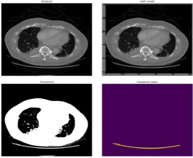
[image:10.595.205.395.278.433.2]In this paper, the CT image of the liver tumor is classified by two CNN networks to realize the image segmentation. The input image is a CT image of three different phases which size is 128*128, including the arterial phase, the portal vein phase and the delayed phase. After preprocessing, the parameters in the network are trained by minimizing the improved cross-entropy loss function. The predicted pixel categories of the three phase image blocks are calculated in CNN-I, in which the parameters are trained from the data from different phases.
Figure 5. CT image of liver tumor after pretreatment.
Then the output pixel class is comprehensively analyzed as the input of CNN-II, and the final output pixel classification is obtained.
EVALUATING INDICATOR
The performance evaluation index of classification task can be described mainly by confusion matrix. The true positive (TP), false positiven (FP), ture negative (TN) and false negative (FN) represent the four categories predicted by the sample and predicted by the mode. And the sum of TP, FP, TN and FN numbers is equal to the number of samples.
TABLEII.TWOCLASSIFICATIONCONFUSIONMATRIX.
Reality
Prediction Result
positive negative
positive TP FN
negative FP TN
[image:10.595.139.442.659.730.2]FN TN FP TP
TN TP accuracy
FP TP
TP precision
FN TP
TP rate
recall
recall precision
recall precision
measure F
2
1
There are great defects in using accuracy as an evaluation index in the case of imbalance between positive and negative samples. The precision measures how likely the model is to predict the correct positive class, and the recall rate measures the extent to which the correct positive class predicted by the model includes a true positive sample. The F1-measure is the harmonic mean value of the precision rate and the recall rate. When the precision rate and recall rate are both high, the F1-measure will also be high. In this paper, the accuracy rate and recall rate are used as evaluation indexes to quantitatively evaluate the results of the automatic segmentation method.
EXPERIMENTAL RESULT
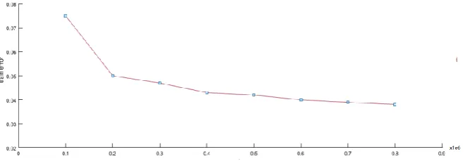
[image:11.595.132.464.440.558.2]In the experiment, the CT image is divided into training set and test set, and the network is trained by the corresponding correct segmentation label of the training set. As shown in Figure 6 , with the increase of the number of iterations in training samples, the error rate of sample classification decreases, and the network model tends to be stable. The test set is automatically segmented by using the trained neural network to evaluate the segmentation performance.
[image:11.595.119.469.611.715.2]Figure 6. Diagram of the Variation of Training Error with the Number of Samples.
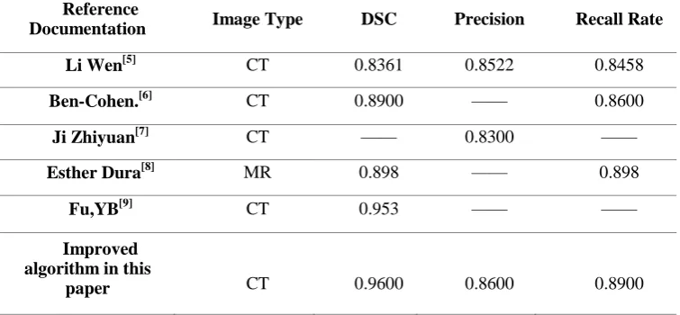
TABLE III. COMPARISON OF THE RESULTS OF DIFFERENT LIVER TUMOR SEGMENTATION METHODS.
Reference
Documentation Image Type DSC Precision Recall Rate
Li Wen[5] CT 0.8361 0.8522 0.8458
Ben-Cohen.[6] CT 0.8900 —— 0.8600
Ji Zhiyuan[7] CT —— 0.8300 ——
Esther Dura[8] MR 0.898 —— 0.898
Fu,YB[9] CT 0.953 —— ——
Improved algorithm in this
paper CT 0.9600 0.8600 0.8900
We obtain the trained parameters to test through the training set input network, and the input test set to obtain the segmented tumor image. The black mark in the Figure 7 shows the location of the tumor that is automatically segmented by the liver tumor.
We used the improved convolutional neural network to segment liver tumors, and the final DC coefficient reached 96%. In terms of accuracy, the calculated value reached 86%.In terms of recall rate, 89%. Compared with other tumor segmentation methods, the result is shown in Table III.
CONCLUSION
In this paper, an automatic segmentation method for CT images of liver tumors based on improved convolution neural network algorithm is proposed. The experimental results show that its quantitative evaluation results are better than those of traditional neural network, and the precision rate and recall rate are 86% and 89% respectively. Therefore, the automatic segmentation method proposed in this paper can provide an objective reference for radiologists to segment liver CT images and a new idea for further research to improve the loss function and use three-phase image training, which is helpful to the rapid development of automatic diagnosis and evaluation of liver tumors.
REFERENCES
1. Li Wen. Liver Tumor Segmentation from 3D CT Images Based on Deep Convolutional
Neural Networks [D]. Shenzhen Institytes of Advanced Technology, 2016.
2. Ben-Cohen A, Diamant I, Klang E, Amitai M, Greenspan H . Fully convolutional
3. Peijun Hu, Fa Wu, Jialin Peng, Ping Liang, Dexing Kong. Automatic 3D liver segmentation based on deep learning and globally optimized surface evolution[J]. Physics in Medicine and Biology, 2016, 61(24).
4. Eli Gibson, Maria R. Robu, Stephen Thompson, P. Eddie Edwards, Crispin Schneider,
Kurinchi Gurusamy, Brian Davidson, David J. Hawkes, Dean C. Barratt, Matthew J. Clarkson. Deep residual networks for automatic segmentation of laparoscopic videos of the liver[P]. Medical Imaging.2017.
5. Kai Hu, Zhenzhen Zhang, Xiaorui Niu, Yuan Zhang, Chunhong Cao, Fen Xiao, Xiepin
Gao. Retinal vessel segmentation of color fundus images using multiscale convolutional neural network with an improved cross-entropy loss function[J]. Neurocomputing, 2018,309.
6. Fu, YB (Fu, Yabo); Mazur, etc. A novel MRI segmentation method using CNN-based
correction network for MRI-guided adaptive radiotherapy[J].Medical Physics. 2018.
7. Ji Zhiyuan. A study on Focal Liver Lesion Classification Based on Multiphase 3D CT
images[D]. Zhejiang University, 2018.
8. Peng Gu, Won-Mean Lee, Marilyn A. Roubidoux, Jie Yuan, Xueding Wang, Paul L.
Carson. Automated 3D ultrasound image segmentation to aid breast cancer image interpretation[J]. Ultrasonics.2016.
9. Tang Yongqiang, Shi Lei, Shu Jun, etc. Imaging features of primary hepatic
neuroendocrine [J]. Chinese Medical Equipment Journal, 2018.
10. https://cancergenome.nih.gov/[DB/OL].2019.
11. Convergence Analysis of BP Algorithm Based on Relative Entropy Function
![Figure 1. Medical imaging of liver tumors in ART, PV and DL[9] .](https://thumb-us.123doks.com/thumbv2/123dok_us/240690.1023742/2.595.197.396.620.688/figure-medical-imaging-liver-tumors-art-pv-dl.webp)