R E S E A R C H
Open Access
A novel approach based on
preference-based index for interval bilevel
linear programming problem
Aihong Ren
1*, Yuping Wang
2and Xingsi Xue
3*Correspondence:
1Department of Mathematics, Baoji
University of Arts and Sciences, Baoji, 721013, China Full list of author information is available at the end of the article
Abstract
This paper proposes a new methodology for solving the interval bilevel linear programming problem in which all coefficients of both objective functions and constraints are considered as interval numbers. In order to keep as much uncertainty of the original constraint region as possible, the original problem is first converted into an interval bilevel programming problem with interval coefficients in both objective functions only through normal variation of interval number and
chance-constrained programming. With the consideration of different preferences of different decision makers, the concept of the preference level that the interval objective function is preferred to a target interval is defined based on the
preference-based index. Then a preference-based deterministic bilevel programming problem is constructed in terms of the preference level and the order relationmw. Furthermore, the concept of a preference
δ
-optimal solution is given. Subsequently, the constructed deterministic nonlinear bilevel problem is solved with the help of estimation of distribution algorithm. Finally, several numerical examples are provided to demonstrate the effectiveness of the proposed approach.Keywords: bilevel programming; interval number; preference-based index; estimation of distribution algorithm
1 Introduction
The bilevel programming problem is a hierarchical optimization problem involving de-cision processes with two dede-cision makers, the so-called leader or upper level dede-cision maker and the so-called follower or lower level decision maker. In such a hierarchical decision framework, the leader first specifies a strategy, and then the follower chooses a strategy in view of the leader’s decision. Two decision makers attempt to optimize their respective objective functions, but are affected by the actions with each other. In the past few decades, the bilevel programming problem has widely applied in numerous areas in-cluding transport network design [, ], price control [], principal-agent problems [, ], supply chain management [, ], engineering design [, ], electricity markets []. Never-theless, the bilevel programming problem is generally non-convex and non-differentiable, and it is NP-hard [] and quite difficult to deal with. Many researchers have worked on this topic, like Dempe [], Colsonet al.[], Kalashnikovet al.[], Bard [], Dempe [], Dempeet al.[] and Zhanget al.[].
It is well known that, in the conventional bilevel programming problem, the coefficients in both objective functions and constraints are deterministic or crisp. However, in prac-tice, we may be faced with some situations where the coefficients in the problem are uncer-tain. To tackle these uncertain coefficients, stochastic and fuzzy approaches are commonly used, and accordingly stochastic and fuzzy bilevel programming problems are proposed. In stochastic bilevel programming problems [], the coefficients are viewed as random variables with known probability distributions; whereas in fuzzy bilevel programming problems [, ], the coefficients are regarded as fuzzy sets with known membership functions. It is worth mentioning that the probability distributions and the membership functions are of great importance to formulate and solve these two classes of problems. However, it is a complicated task for decision makers to choose appropriate probability distributions or membership functions in the case of stochastic or fuzzy uncertainties. To efficiently cope with the uncertainties, there emerges the interval programming, which becomes a prominent tool for tackling decision problems with uncertain parameters and it only requires to calculate the bounds of the uncertain coefficients. On this basis, the interval bilevel programming problem, whose coefficients of both objective functions or constraints are interval numbers, begins to attract more and more researchers, but to the best of our knowledge, academic papers about this kind of problem are still few.
Under the above consideration, from a point of decision makers’ preferences, our ob-jective is to propose an alternative way based on preference-based index to deal with the interval bilevel linear programming problem in which all coefficients in both objective functions and constraints are intervals. To this end, we first convert the original constraint region into its crisp equivalent form by combining normal variation of interval number with chance-constrained programming [], and thus transform the original problem into an interval bilevel programming problem where interval coefficients are in both objective functions only. This kind of transformation keeps the uncertainty of the original constraint region as much as possible. Taking into account different preferences of different decision makers, the preference level that the interval objective function is preferred to a target interval is defined in terms of preference-based index developed by Ruanet al.[]. Then a preference-based deterministic bilevel programming problem can be constructed by re-placing the upper level interval objective function with corresponding preference level and using the order relationmwto handle the lower level interval objective function. For
the constructed nonlinear deterministic problem, we adopt an estimation of distribution algorithm to solve it. Finally, several numerical examples are provided to demonstrate the feasibility of the proposed method.
The remainder of this paper is organized as follows. Section briefly recalls some ba-sic definitions and preliminary results related to interval numbers. In Section , we intro-duce the interval bilevel linear programming problem. In Section , a new approach based on preference-based index is proposed to handle the interval bilevel linear programming problem. Section provides some numerical examples to illustrate the proposed method and make some comparisons with the existing methods. Finally, we conclude the paper and suggest directions for future work in Section .
2 Preliminaries
LetRbe the set of all real numbers. An interval numbercIcan be defined as
cI=c–,c+=c|c–≤c≤c+,c∈R,
wherec–andc+are the lower and upper bounds ofcI, respectively. Ifc–=c+, thencI is a real number.
In terms of its midpoint and half-width, an interval numbercI can also be defined as
cI=mcI,wcI =c|mcI–wcI≤c≤mcI+wcI,c∈R, wherem(cI) =c–+c+
andw(cI) =
c+–c–
are the midpoint and half-width of intervalcI,
re-spectively. ForcI
= [c–,c+],cI= [c–,c+] andcI= [c–,c+], the arithmetical operations on intervals are
defined as follows:
(i) cI
+cI= [c– +c–,c++c+]; (ii) cI
–cI= [c– –c+,c+–c–]; (iii) kcI=[kc–,kc+], k≥,
[kc+,kc–, ] k< .
With respect to the more details of interval mathematics, please see Moore [] and Alefeld and Herzberger [].
Definition ([]) The order relationmwbetween two interval numberscI= [c–,c+] and cI
= [c–,c+] is defined as: cI
mwcIifm(cI)≤m(cI) andw(cI)≤w(cI) for minimization problems, cI
mwcIifm(cI)≤m(cI) andw(cI)≥w(cI) for maximization problems.
Furthermore,cI
≺mwcIifcImwcIandcI=cI.
Definition ([]) The perceived value of an interval numbercI= [c–,c+] is defined as:
ocI=γc–+ ( –γ)c+,
whereγ(≤γ ≤) is the optimism degree of decision makers.
Definition ([]) For any two interval numberscI
= [c–,c+] andcI= [c–,c+], a
prefer-ence-based index can be defined as:
δcI≺cI= o(c
I
) –o(cI) w(c
) +w(cI) +
=(γc
–
+ ( –γ)c+) – (γc– + ( –γ)c+)
(c +
–c–) +(c +
–c–) +
,
where≺denotescI
to be inferior tocI,o(cI) ando(cI) denote the perceived values ofcI
andcI
, respectively. Ifδ(cI≺cI) > ,cIis preferred tocIfor a minimization problem. 3 Interval bilevel linear programming problem
Consider the following interval bilevel linear programming problem with interval objec-tives and interval constraints:
⎧ ⎪ ⎪ ⎪ ⎪ ⎪ ⎪ ⎪ ⎪ ⎨ ⎪ ⎪ ⎪ ⎪ ⎪ ⎪ ⎪ ⎪ ⎩
minx [c–,c+]x+ [c–,c+]x
wherexsolves
minx [c–,c+]x+ [c–,c+]x
s.t. [a–
i,a+i]x+ [a–i,ai+]x≥[bi–,b+i], i= , , . . . ,m,
x≥,x≥,
()
wherexandxaren-dimensional upper level decision variable column vector andn
-dimensional lower level decision variable column vector, respectively, [c–
lj,c+lj], l,j= , ,
and [a–
ij,a+ij],i= , , . . . ,m, arenj-dimensional interval vectors whose components are all
intervals, and [b–
i,b+i],i= , , . . . ,mare interval numbers.
Here, it is important to realize that the meaning of minimizing both objective functions and inequality constraints is not clear at all owing to the presence of interval coefficients in problem (). In other words, how to tackle the relationship between the left and the right hand sides of the interval inequality constraints and how to search the optimal values for the interval objective functions are two important issues. Thus we cannot blindly apply solution concepts and existing approaches for deterministic bilevel cases to handle this type of problem. For this purpose, we will develop a solution methodology from a new perspective to transform and deal with problem () in the following section.
4 Solution methodology
4.1 Conversion of the interval constraint region into its crisp one
To deal with problem (), we first shall discuss crisp equivalent transformation for the in-terval constraint region in problem (). In order to do so, we first need to convert each interval inequality constraint into its crisp form. From the point of decision maker’s satis-faction, several typical methods introduced by Senguptaet al.[], Guo and Wu [], and Allahdadi and Nehi [] mainly focus on transforming an interval inequality constraint into a type of satisfactory crisp constraint. However, it has been pointed out by Chenet al.
[] that these types of conversion could lose the uncertainty of intervals in part during the transformation process. In a different approach, recently Chenet al.[] discussed a new equivalent transformation for interval inequality constraint in terms of normal variation of interval number and chance-constrained programming approach. The main advantage of this kind of transformation is to maintain as much uncertainty as possible. In this way, we first transform any interval inequality constraint of problem () into a stochastic in-equality form by normal variation of intervals.
For any intervalaI = [a–,a+], in terms of the σ law, its corresponding normally
dis-tributed random variable, denoted bya¯∼N(μ,σ), can be determined as follows:
μ=a
–+a+
, σ=
a+–a–
.
Clearly, we have [a–,a+] = [μ– σ,μ+ σ]. Notice that the probability that any interval numbera¯ falls in [a–,a+] is .%on the basis of the σ law. Thus it is reasonable to utilize a normally distributed random variable to represent an interval.
By replacing interval coefficients with their corresponding normally distributed random variables, theith interval inequality constraint of problem () can be converted as:
¯
aix+a¯ix≥ ¯bi, i= , , . . . ,m,
where a¯ij = (a¯ij,a¯ij, . . . ,a¯ijnj), i = , , . . . ,m, j= , , are corresponding normally
dis-tributed random vectors of interval vectors [a–ij,a+ij], andb¯i,i= , , . . . ,mare
correspond-ing normally distributed random variables of interval numbers [b–i,b+i]. For simplicity, we assume thata¯ij,a¯ij, . . . ,a¯ijnjandb¯iare independent from each other.
As is well known, chance-constrained programming approach [] is the most applied one to handle the stochastic constraints. By this means, stochastic constraints hold at least some satisficing probability level specified by decision makers. With the aid of chance-constrained programming, the aboveith stochastic inequality constraint can be reformu-lated as follows:
Pr{¯aix+a¯ix≥ ¯bi} ≥βi, i= , , . . . ,m,
wherePrdenotes the probability of the event, andβi∈(, ) is the probability level of the
ith constraint,i= , , . . . ,m.
Now we have converted the interval constraint region of problem () into its crisp struc-ture. Then problem () can be transformed into the following problem:
⎧ ⎪ ⎪ ⎪ ⎪ ⎪ ⎪ ⎪ ⎪ ⎪ ⎪ ⎪ ⎪ ⎪ ⎪ ⎪ ⎪ ⎪ ⎨ ⎪ ⎪ ⎪ ⎪ ⎪ ⎪ ⎪ ⎪ ⎪ ⎪ ⎪ ⎪ ⎪ ⎪ ⎪ ⎪ ⎪ ⎩
minx [c–
,c+]x+ [c–,c+]x
wherexsolves
minx [c–,c+]x+ [c–,c+]x
s.t. n
s=E(a¯is)xs
+n
t=E(a¯it)xt
+–(βi)
n
s=V(a¯is)xs+
n
t=V(a¯it)xt+V(b¯i)
≥E(b¯i), i= , , . . . ,m,
x= (x,x, . . . ,xn)T≥,x= (x,x, . . . ,xn)T≥,
()
whereE(·) andV(·) denote the expectation and variance of a random variable, and–is the inverse function of standardized normal distribution.
For convenience, we denote the constraint region of problem () byD. Equivalently, problem () can be rewritten as
⎧ ⎪ ⎪ ⎪ ⎪ ⎪ ⎨ ⎪ ⎪ ⎪ ⎪ ⎪ ⎩
minx F
I(x,x) = [c–
,c+]x+ [c–,c+]x
wherexsolves
minx f
I(x,x) = [c–
,c+]x+ [c–,c+]x
s.t. (x,x)∈D,
()
whereFI= [F–,F+] andfI= [f–,f+] denote interval objective functions of the upper and
lower level programming problems, respectively.
Clearly, the above problem is a bilevel programming problem with interval coefficients in both objective functions only.
4.2 Preference-based deterministic bilevel programming problem
In order to reflect different preferences of different decision makers, in this section we first introduce the concept of the preference level that the interval objective function is preferred to a target interval in light of preference-based index in []. Then we build a preference-based deterministic bilevel programming problem for problem () based on the preference level and the order relationmw.
For a given x, the lower level programming problem of problem () is an essentially single level optimization problem for objective function involving interval coefficients. For this type of problem, the midpoints of the intervals are often used to cope with the related interval objective functions, but it may cause the loss of helpful information to some extent in terms of such a treatment. To better reflect uncertain information, the order relation≤mwwhich considers the midpoint and half-width of intervals at the same
level problem can be converted into the following problem:
⎧ ⎨ ⎩
minx θm(fI(x
,x)) + ( –θ)w(fI(x,x))
x∈D(x), ()
whereθ(≤θ≤) denotes a weighting factor,m(fI(x
,x)) = f
–(x
,x)+f+(x,x)
andw(f
I(x
, x)) = f
+(x
,x)–f–(x,x)
represent the midpoint and half-width of the lower level objective
functionfI(x
,x), respectively.
Denote the set of optimal solutions of problem () byMI(x
) for a givenx. Then the
feasible region of problem () can be defined as:
IRI=(x,x)|(x,x)∈D,x∈MI(x). Thus problem () can be formulated as:
⎧ ⎨ ⎩
minx,x FI(x,x)
s.t. (x,x)∈IRI.
()
It is well known that the order relation between intervals is often applied to tackle inter-val objective function. So far there have been all sorts of definitions of the interinter-val order relations based on various mathematical approaches [–] with the exception of the order relationmwmentioned above. Among them, Sengupta and Pal [] proposed the
acceptability index for ranking any two interval numbers based on decision maker’s sat-isfaction. It has been pointed out by Ruanet al.[] that this index cannot be applied for reflecting different preferences from different decision makers. For this purpose, we ap-ply preference-based index for ranking interval numbers introduced by Ruanet al.[] to treat the interval objective function in the upper level of problem ().
In order to find a satisfying solution for the decision maker at the upper level, the interval objective function often needs to satisfy a desired target interval determined in advance by the decision maker as far as possible. LetCI= [C–,C+] be a predetermined target interval corresponding to the upper level objective function. Based on preference-based index for ranking interval numbers, we define the concept of the preference level as follows.
Definition For any (x,x)≥,δ(FI(x,x)≺CI) is said to be a preference level that
the interval objective functionFI(x,x) is inferior to a target intervalCI. Ifδ(FI(x,x)≺
CI) > ,FI(x,x) is preferred toCI for a minimization problem.
Clearly, it needs to maximize the preference level of the interval objective function to be inferior to its target interval for a minimization problem. In this sense, problem () can be transformed into the following preference-based deterministic bilevel programming problem:
⎧ ⎨ ⎩
maxx,x δ(FI(x,x)≺CI)
s.t. (x,x)∈IRI.
()
Definition A solution (x∗,x∗)∈IRIis said to be a preferenceδ-optimal solution of
prob-lem () if there does not exist another feasible solution (x,x)∈IRIsuch thatδ(FI(x,x)≺
CI)≥δ(FI(x∗,x∗)≺CI).
Using Definition , we have
δFI(x,x)≺CI
= o(C
I) –o(FI(x,x))
w(CI) +w(FI(x,x)) + .
Thus problem () can be rewritten as
⎧ ⎪ ⎪ ⎪ ⎪ ⎪ ⎪ ⎪ ⎪ ⎪ ⎪ ⎪ ⎪ ⎪ ⎪ ⎪ ⎪ ⎪ ⎨ ⎪ ⎪ ⎪ ⎪ ⎪ ⎪ ⎪ ⎪ ⎪ ⎪ ⎪ ⎪ ⎪ ⎪ ⎪ ⎪ ⎪ ⎩
maxx
o(CI)–o(FI(x
,x))
w(CI)+w(FI(x
,x))+
wherexsolves
minx θm(fI(x,x)) + ( –θ)w(fI(x,x))
n
s=E(a¯is)xs
+n
t=E(a¯it)xt
+–(βi)
n
s=V(a¯is)xs+
n
t=V(a¯it)xt+V(b¯i)
≥E(b¯i), i= , , . . . ,m,
x= (x,x, . . . ,xn)T≥,x= (x,x, . . . ,xn)T≥.
()
On the other hand, if the original problem is a type of maximization stated as follows:
⎧ ⎪ ⎪ ⎪ ⎪ ⎪ ⎪ ⎪ ⎪ ⎨ ⎪ ⎪ ⎪ ⎪ ⎪ ⎪ ⎪ ⎪ ⎩
maxx [c–,c+]x+ [c–,c+]x
wherexsolves
maxx [c–,c+]x+ [c–,c+]x
s.t. [a–i,ai+]x+ [a–i,a+i]x≥[bi–,b+i], i= , , . . . ,m,
x≥,x≥.
()
For problem (), the decision maker hopes to maximize the preference level of the
inter-val objective function to be superior to its target interinter-val. By using the similar idea for the
above minimization, another preference-based deterministic bilevel programming
prob-lem of probprob-lem () can be expressed as:
⎧ ⎪ ⎪ ⎪ ⎪ ⎪ ⎨ ⎪ ⎪ ⎪ ⎪ ⎪ ⎩
maxx δ(FI(x,x)CI)
wherexsolves
maxx θm(fI(x,x)) + ( –θ)(–w(fI(x,x)))
(x,x)∈D.
Equivalently, problem () can be rewritten in the form
⎧ ⎪ ⎪ ⎪ ⎪ ⎪ ⎪ ⎪ ⎪ ⎪ ⎪ ⎪ ⎪ ⎪ ⎪ ⎪ ⎪ ⎪ ⎨ ⎪ ⎪ ⎪ ⎪ ⎪ ⎪ ⎪ ⎪ ⎪ ⎪ ⎪ ⎪ ⎪ ⎪ ⎪ ⎪ ⎪ ⎩
maxx o(FI(x,x))–o(CI)
w(FI(x,x))+w(CI)+
wherexsolves
maxx θm(f
I(x,x)) + ( –θ)(–w(fI(x,x)))
n
s=E(a¯is)xs
+n
t=E(a¯it)xt
+–(β
i)ns= V(a¯is)xs+
n
t=V(a¯it)xt+V(b¯i)
≥E(b¯i), i= , , . . . ,m,
x= (x,x, . . . ,xn)
T≥,x
= (x,x, . . . ,xn)
T≥.
()
Clearly, problems () and () are a class of nonlinear bilevel programming problems which are coped with by one of the metaheuristic techniques namely estimation of distri-bution algorithm in the next subsection.
4.3 Solution approach based on estimation of distribution algorithm
It is well known that bilevel programming problem is a complex optimization model and it is difficult to tackle. Usually, traditional solution methods involve huge computational load when solving this type of problem and they are only successful for some special bilevel cases. Estimation of distribution algorithm (EDA) [], which is a new evolutionary meta-heuristic algorithm, has attracted considerable attention as an alternative method for solv-ing bilevel programmsolv-ing problem [, ] in recent years. For EDA, the main steps of the iterative procedure include: randomly create initial population, select some excellent in-dividuals, build a probabilistic model based on excellent individuals chosen, generate new individuals by sampling from the constructed probabilistic model, and repeat the cycle until a stopping criterion is met. Notice that the main characteristics of this approach is to reproduce a new generation implicitly by sampling from a probability model constructed by promising candidate solutions.
In our work, estimation of distribution algorithm is applied to solve nonlinear bilevel programming problems () and (). For these two problems, observing that the lower level objective functions are linear and constraint functions are quadratic, thus a number of traditional techniques can be employed to solve the lower level problem. Furthermore, estimation of distribution algorithm is used to deal with the upper level problem. Based on these ideas, we give the details of the computational method by combining estimation of distribution algorithm with some traditional method for solving problems () and () as follows:
Step Ask the decision makers to specify the probability levelsβi,i= , , . . . ,m,
weighting factorθ, target intervalCI and optimism degree of the upper level
decision makerγ. Generate the initial populationPop()with population sizeN comprised by the upper level decision variable. Lett= .
Step For each given upper level individual, we solve the lower level problem by means of some traditional method.
Step SelectMbest individuals fromPop(t)to form the parent setQ(t)by the truncation selection, and update the probability model by estimating the distribution ofQ(t).
Step SampleNnew individuals from the updated probabilistic model. Denote the set of all these individuals byO(t). SelectNbest offspring candidates from the set
Pop(t)∪O(t)to construct the next populationPop(t+ ).
Step If the algorithm is executed to the maximal number of generations, then stop; otherwise, lett=t+ , go to Step .
5 Numerical examples and discussion
To show the feasibility and efficiency of the proposed approach for handling the interval bilevel linear programming problem, we test three numerical examples in this section. Furthermore, some comparisons between the proposed method and some existing ap-proaches are made to better demonstrate advantages of the proposed approach.
5.1 Numerical examples
The following three examples are selected from the existing literature.
Example This example extracted from the literature [] is an interval bilevel linear
programming problem with only one interval inequality constraint:
⎧ ⎪ ⎪ ⎪ ⎪ ⎪ ⎪ ⎪ ⎪ ⎪ ⎪ ⎪ ⎨ ⎪ ⎪ ⎪ ⎪ ⎪ ⎪ ⎪ ⎪ ⎪ ⎪ ⎪ ⎩
maxx [, ]x+ [, ]y
whereysolves
maxy [, ]x+ [, ]y
s.t. [, ]x+ [, ]y≥,
x+y≤,
x≥,y≥.
()
Example The following interval bilevel linear programming problem in which all the
coefficients in constraints are interval numbers is taken from []:
⎧ ⎪ ⎪ ⎪ ⎪ ⎪ ⎪ ⎪ ⎪ ⎪ ⎪ ⎪ ⎪ ⎪ ⎪ ⎪ ⎪ ⎪ ⎪ ⎪ ⎪ ⎨ ⎪ ⎪ ⎪ ⎪ ⎪ ⎪ ⎪ ⎪ ⎪ ⎪ ⎪ ⎪ ⎪ ⎪ ⎪ ⎪ ⎪ ⎪ ⎪ ⎪ ⎩
minx [, ]x+ [–, ]y
whereysolves
miny [, ]y
s.t. [, ]x+ [, ]y≥[,], [–, –]x+ [, ]y≥[–, –], [–, –]x+ [, ]y≥[–, –], [–, –]x+ [–, –]y≥[–, – ], [, ]x+ [–, –]y≥[–, –],
x≥,y≥.
Table 1 Normal distributions corresponding to interval coefficients in the first constraint of Example 1
Interval N(μ,σ2) Interval N(μ,σ2)
[image:11.595.118.480.297.364.2][3, 5] N(4, 0.33332) [4, 6] N(5, 0.33332)
Table 2 Normal distributions corresponding to interval coefficients in all the constraints of Example 2
Interval N(μ,σ2) Interval N(μ,σ2) Interval N(μ,σ2)
[3435, 1] N(0.9857, 0.00482) [17
10, 2] N(1.85, 0.052) [10, 51
5] N(10.1, 0.03332) [–7
6, –1] N(–1.0833, 0.0278 2) [7
5, 2] N(1.7, 0.1
2) [–6, –161
30] N(–5.6833, 0.1056 2)
[–5
2, –2] N(–2.25, 0.0833
2) [1
2, 1] N(0.75, 0.0833
2) [–21, –20] N(–20.5, 0.16672)
[–63
40, –1] N(–1.2875, 0.0958
2) [–21
10, –2] N(–2.05, 0.0167
2) [–38, –1407
40 ] N(–36.5875, 0.4708 2)
[157, 1] N(0.7333, 0.08892) [–2110, –2] N(–2.05, 0.01672) [–18, –845] N(–17.4, 0.22)
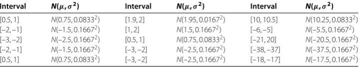
Table 3 Normal distributions corresponding to interval coefficients in all the constraints of Example 3
[image:11.595.137.312.431.584.2]Interval N(μ,σ2) Interval N(μ,σ2) Interval N(μ,σ2)
[0.5, 1] N(0.75, 0.08332) [1.9, 2] N(1.95, 0.01672) [10, 10.5] N(10.25, 0.08332) [–2, –1] N(–1.5, 0.16672) [1, 2] N(1.5, 0.16672) [–6, –5] N(–5.5, 0.16672) [–3, –2] N(–2.5, 0.16672) [0.5, 1] N(0.75, 0.08332) [–21, 20] N(–20.5, 0.16672) [–2, –1] N(–1.5, 0.16672) [–3, –2] N(–2.5, 0.16672) [–38, –37] N(–37.5, 0.16672) [0.5, 1] N(0.75, 0.08332) [–3, –2] N(–2.5, 0.16672) [–18, –17] N(–17.5, 0.16672)
Example Consider the following interval bilevel linear programming problem from
[]:
⎧ ⎪ ⎪ ⎪ ⎪ ⎪ ⎪ ⎪ ⎪ ⎪ ⎪ ⎪ ⎪ ⎪ ⎪ ⎪ ⎪ ⎪ ⎪ ⎪ ⎪ ⎨ ⎪ ⎪ ⎪ ⎪ ⎪ ⎪ ⎪ ⎪ ⎪ ⎪ ⎪ ⎪ ⎪ ⎪ ⎪ ⎪ ⎪ ⎪ ⎪ ⎪ ⎩
minx [–, –.]y
whereysolves
miny [, ]y
s.t. [., ]x+ [., ]y≥[, .], [–, –]x+ [, ]y≥[–, –], [–, –]x+ [., ]y≥[–, –], [–, –]x+ [–, –]y≥[–, –], [., ]x+ [–, –]y≥[–, –],
x≥,y≥.
()
5.2 Results and discussion
In this section, we show the computational results of three numerical examples to assess the performance of the proposed approach. The parameters, population size of each gen-eration, size of the selected population, maximum number of generations, associated with estimation of distribution algorithm are taken as , and , respectively.
equivalent forms. For simplicity, each chance-constrained probability related to the
re-sulted stochastic inequality constraints is set as β= ., and we have–(β) = ..
Based on the proposed models () and (), these interval bilevel linear programming
problems can be converted into their equivalent deterministic ones.
For Example , the interval target corresponding to the upper level objective functions
are set asCI = [, ], and the weighting factor for the lower level objective function is
set asθ = .. On the basis of model (), then the equivalent deterministic form of this
problem is expressed as follows:
⎧ ⎪ ⎪ ⎪ ⎪ ⎪ ⎪ ⎪ ⎪ ⎪ ⎪ ⎪ ⎪ ⎨ ⎪ ⎪ ⎪ ⎪ ⎪ ⎪ ⎪ ⎪ ⎪ ⎪ ⎪ ⎪ ⎩
maxx [γ(x+y()+(–x+y)–(γ)(xx++y)y)]–[γ+(–γ)] +– +
whereysolves
maxy .[(x+y)+( x+y)] + .[–(x+y)–( x+y)]
s.t. x+ y+ ..x+ .y≥, x+y≤,
x≥,y≥.
()
We apply estimation of distribution algorithm to solve model () with assumption that
the decision makers specify the optimism degreeγ = .. Then we obtain the following
result: the optimal solution is (x∗,y∗) = (, ), the corresponding upper level objective value
isF.I = [, ]. Furthermore, we haveδ(F.I [, ]) = .. This indicates that the obtained interval value of the upper level objective function is superior to the interval
goal.
For this example, Abass [] gives the optimal solution as (x∗,y∗) = (, ) with the
pos-sibility degree levelλ= . by adopting the midpoints and half-widths of the interval
co-efficients to formulate both interval objective functions and applying the concept of the
possibility degree of interval number to treat interval inequality constraints. As far as the
final result is concerned, the result obtained by our approach is the same as that obtained
in []. From the viewpoint of equivalent transformation of interval inequality constraint,
our approach can ensure that the formulated stochastic constraint at the obtained optimal
solution holds with probability of at least % based on chance-constrained
program-ming, in other words, this constraint is violated with probability of at most %. While
equivalent conversion based on the possibility degree of interval number in [] holds at
a small possibility degree levelλ= .. As we know, a smaller possibility degree means a
lower reliability of the interval constraint. Thus the result obtained by Abass’ approach
[] shows a relatively low reliability.
For Example , the interval goal is set asCI= [, ] for the upper level objective
the equivalent deterministic bilevel problem can be stated as follows: ⎧ ⎪ ⎪ ⎪ ⎪ ⎪ ⎪ ⎪ ⎪ ⎪ ⎪ ⎪ ⎪ ⎪ ⎪ ⎪ ⎪ ⎪ ⎪ ⎪ ⎪ ⎪ ⎪ ⎪ ⎨ ⎪ ⎪ ⎪ ⎪ ⎪ ⎪ ⎪ ⎪ ⎪ ⎪ ⎪ ⎪ ⎪ ⎪ ⎪ ⎪ ⎪ ⎪ ⎪ ⎪ ⎪ ⎪ ⎪ ⎩
maxx [γ+(––γ)]–[γ(–y)+(–γ)(x+y)] +
(x+y)–(–y)
+
whereysolves
miny .(y+y) + .(y–y)
s.t. .x+ .y+ ..x+ .y+ .≥.,
–.x+ .y+ ..x+ .y+ .≥–.,
–.x+ .y+ ..x+ .y+ .≥–.,
–.x– .y+ ..x+ .y+ . ≥–.,
.x– .y+ ..x+ .y+ .≥–., x≥,y≥.
()
Next, we cope with the above problem by estimation of distribution algorithm with
γ = .. The optimal solution is (x∗,y∗) = (., .) and the corresponding upper level objective value isFI
.= [–., .]. Also, we obtainδ(F.I ≺[, ]) = .. Thus FI
.is preferred toCI at preference-based index ..
By using two types of cutting plane methods developed by Ren and Wang [], the best and worst optimal solutions of this example is finally obtained as (, ) and (, ), and the corresponding upper objective function values are [–, ] and [–, ]. In the light of preference-based index,δ([–, ].≺[, ]) = . andδ([–, ].≺[, ]) =
. whenγ= .. It is obvious that a modest optimal interval value of the upper level is offered to an optimistic decision maker.
For Example , the interval goal corresponding to the upper level objective function is specified asCI= [–, ], and the weighting factor related to the lower level objective
function is chosen asθ = .. Then problem () can be transformed into the following equivalent deterministic bilevel problem by making use of model ():
⎧ ⎪ ⎪ ⎪ ⎪ ⎪ ⎪ ⎪ ⎪ ⎪ ⎪ ⎪ ⎪ ⎪ ⎪ ⎪ ⎪ ⎪ ⎪ ⎪ ⎪ ⎨ ⎪ ⎪ ⎪ ⎪ ⎪ ⎪ ⎪ ⎪ ⎪ ⎪ ⎪ ⎪ ⎪ ⎪ ⎪ ⎪ ⎪ ⎪ ⎪ ⎪ ⎩
maxx [γ(–)+(––(–)γ)]–[γ(–y)+(–γ)(x+y)]
+
(x+y)–(–y)
+
whereysolves
miny .(y+y) + .(y–y)
s.t. .x+ .y+ ..x+ .y+ .≥.
–.x+ .y+ ..x+ .y+ .≥–.
–.x+ .y+ ..x+ .y+ .≥–.
–.x– .y+ ..x+ .y+ .≥–.
.x– .y+ ..x+ .y+ .≥–. x≥,y≥.
()
After solving the above problem by estimation of distribution algorithm atγ = ., we obtain its optimal solution (x∗,y∗) = (., .) and the corresponding upper level objective valueFI
.= [–., –.]. Meanwhile, we get δ(F.I ≺[–, ]) = ..
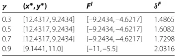
Table 4 Objection function values and corresponding preference-based indices under different optimism degrees of Example 3
γ (x∗, y∗) FI δF
0.3 [12.4317, 9.2434] [–9.2434, –4.6217] 1.4865 0.5 [12.4317, 9.2434] [–9.2434, –4.6217] 1.6082 0.7 [12.4317, 9.2434] [–9.2434, –4.6217] 1.7298 0.9 [9.1441, 11.0] [–11, –5.5] 2.0316
The best and worst optimal solutions to Example obtained in [] are (, ) and (., .), and corresponding upper level objective values are [–, –.] and [–., –.]. According to preference-based index, when γ = ., we have δ([–, –.]. ≺[–, ]) = . and δ([–., –.].≺[–, ]) = .. Clearly, our
ap-proach provides a modest optimal interval value for an optimistic decision maker of the upper level.
In order to show the influence of different optimism degrees from different decision makers, Table provides the results of the upper level objective function and preference-based index under different optimism degrees. From Table , it is seen thatγ = . has great influence on the upper level objective function. Although the objective function values are unchanged when γ = ., . and ., the corresponding preference-based indices are different. Clearly, pessimistic decision maker (γ = .), moderate decision maker (γ = .) and optimistic decision maker (γ = .) think that the interval value [–., –.] is superior to the interval goalCI
with a lower, moderate and greater
preference-based index.
6 Conclusions
In this paper, we focus on a class of interval bilevel linear programming problems where all coefficients are interval numbers. To deal with these problems, a novel approach based on preference-based index is presented. In particular, we first transform the original prlem into an interval bilevel programming probprlem with interval coefficients in both ob-jective functions only by combining normal variation of interval number with chance-constrained programming. This type of conversion is able to keep the uncertainty of the original constraint region to a larger extent. Then we construct a preference-based de-terministic bilevel programming problem by means of the preference level and the order relationmw. Subsequently, we apply an estimation of distribution algorithm to deal with
the deterministic nonlinear bilevel one. Finally, the experimental results show the effec-tiveness of the presented approach.
As future work, the proposed approach will be applicable to more realistic applications. In addition, we will extend the proposed method to deal with interval bilevel nonlinear programming problems.
Competing interests
The authors declare that they have no competing interests.
Authors’ contributions
Author details
1Department of Mathematics, Baoji University of Arts and Sciences, Baoji, 721013, China.2School of Computer Science
and Technology, Xidian University, Xi’an, 710071, China. 3College of Information Science and Engineering, Fujian
Provincial Key Laboratory of Big Data Mining and Applications, Fujian University of Technology, Fuzhou, 350118, China.
Acknowledgements
This work was supported by National Natural Science Foundation of China (No. 61602010) and Science Foundation of Baoji University of Arts and Sciences (No. ZK16049).
Publisher’s Note
Springer Nature remains neutral with regard to jurisdictional claims in published maps and institutional affiliations.
Received: 9 February 2017 Accepted: 25 April 2017
References
1. Gzara, F: A cutting plane approach for bilevel hazardous material transport network design. Oper. Res. Lett.41(1), 40-46 (2013)
2. Fontaine, P, Minner, S: Benders decomposition for discrete-continuous linear bilevel problems with application to traffic network design. Transp. Res., Part B, Methodol.70, 163-172 (2014)
3. Labbé, M, Violin, A: Bilevel programming and price setting problems. 4OR11(1), 1-30 (2013)
4. Cecchini, M, Ecker, J, Kupferschmid, M, Leitch, R: Solving nonlinear principal-agent problems using bilevel programming. Eur. J. Oper. Res.230(2), 364-373 (2013)
5. Xu, MW, Ye, JJ: A smoothing augmented Lagrangian method for solving simple bilevel programs. Comput. Optim. Appl.59(1), 353-377 (2014)
6. Kis, T, Kovács, A: Exact solution approaches for bilevel lot-sizing. Eur. J. Oper. Res.226(2), 237-245 (2013) 7. Wang, DP, Du, G, Jiao, RJ, Wu, R, Yu, JP, Yang, D: A Stackelberg game theoretic model for optimizing product family
architecting with supply chain consideration. Int. J. Prod. Econ.172, 1-18 (2016)
8. Camacho-Vallejo, JF, Cordero-Franco, AE, González-Ramírez, RG: Solving the bilevel facility location problem under preferences by a Stackelberg-evolutionary algorithm. Math. Probl. Eng.2014, Article ID 430243 (2014)
9. Kalashnikov, V, Matis, TI, Camacho-Vallejo, JF, Kavun, SV: Bilevel programming, equilibrium, and combinatorial problems with applications to engineering. Math. Probl. Eng.2015Article ID 490758 (2015)
10. Zhang, GQ, Zhang, GL, Gao, Y, Lu, J: Competitive strategic bidding optimization in electricity markets using bilevel programming and swarm technique. IEEE Trans. Ind. Electron.58(6), 2138-2146 (2011)
11. Bard, JF: Some properties of the bilevel linear programming. J. Optim. Theory Appl.68(2), 146-164 (1991) 12. Dempe, S: Annotated bibliography on bilevel programming and mathematical programs with equilibrium
constraints. Optimization52(3), 333-359 (2003)
13. Colson, B, Marcotte, P, Savard, G: An overview of bilevel optimization. Ann. Oper. Res.153(1), 235-256 (2007) 14. Kalashnikov, VV, Dempe, S, Pérez-Valdés, GA: Bilevel programming and applications. Math. Probl. Eng.2015Article ID
310301 (2015)
15. Bard, JF: Practical Bilevel Optimization: Algorithms and Applications. Kluwer, Dordrecht (1998) 16. Dempe, S: Foundations of Bilevel Programming. Kluwer, Dordrecht (2002)
17. Dempe, S, Kalashnikov, V, Pérez-Valdés, GA, Kalashnykova, N: Bilevel Programming Problems: Theory, Algorithms and Applications to Energy Networks. Springer, Berlin (2015)
18. Zhang, GQ, Lu, J, Gao, Y: Multi-Level Decision Making: Models, Methods and Applications. Springer, Berlin (2015) 19. Kosuch, S, Le Bodic, P, Leung, J, Lisser, A: On a stochastic bilevel programming problem. Networks59(1), 107-116
(2012)
20. Zhang, GQ, Lu, J: The definition of optimal solution and an extended Kuhn-Tucker approach for fuzzy linear bilevel programming. IEEE Comput. Intell. Bull.5, 1-7 (2005)
21. Zhang, GQ, Lu, J, Dillon, T: Fuzzy linear bilevel optimization: solution concepts, approaches and applications. Stud. Fuzziness Soft Comput.215, 351-379 (2007)
22. Abass, SA: An interval number programming approach for bilevel linear programming problem. Int. J. Manag. Sci. Eng. Manag.5(6), 461-464 (2010)
23. Wang, JZ, Du, G: Research on the method for interval linear bi-level programming based on a partial order on intervals. In: 2011 Eighth International Conference on Fuzzy Systems and Knowledge Discovery pp. 682-686. IEEE, Shanghai (2011)
24. Calvete, HI, Galé, C: Linear bilevel programming with interval coefficients. J. Comput. Appl. Math.236(15), 3751-3762 (2012)
25. Ren, AH, Wang, YP: A cutting plane method for bilevel linear programming with interval coefficients. Ann. Oper. Res.
223, 355-378 (2014)
26. Nehi, HM, Hamidi, F: Upper and lower bounds for the optimal values of the interval bilevel linear programming problem. Appl. Math. Model.39(5-6), 1650-1664 (2015)
27. Chen, MZ, Wang, SG, Wang, PP, Ye, XX: A new equivalent transformation for interval inequality constraints of interval linear programming. Fuzzy Optim. Decis. Mak.15(2), 155-175 (2016)
28. Ruan, JH, Shi, P, Lim, CC, Wang, XP: Relief supplies allocation and optimization by interval and fuzzy number approaches. Inf. Sci.303, 15-32 (2015)
29. Moore, RE, Kearfott, RB, Cloud, MJ: Introduction to Interval Analysis. SIAM, Philadelphia (2009) 30. Alefeld, G, Herzberger, J: Introduction to Interval Computations. Academic Press, New York (1983)
31. Ishibuchi, H, Tanaka, H: Multiobjective programming in optimization of the interval objective function. Eur. J. Oper. Res.48, 219-225 (1990)
33. Sengupta, A, Pal, TK, Chakraborty, D: Interpretation of inequality constraints involving interval coefficients and a solution to interval linear programming. Fuzzy Sets Syst.119(1), 129-138 (2001)
34. Guo, JP, Wu, YH: Standard form of interval linear programming and its solution. Syst. Eng.3, 79-82 (2003) 35. Allahdadi, M, Nehi, HM: The optimal solution set of the interval linear programming problems. Optim. Lett.7(8),
1893-1911 (2013)
36. Charnes, A, Cooper, WW: Chance-constrained programming. Manag. Sci.6, 73-79 (1959)
37. Chanas, S, Kuchta, D: Multiobjective programming in optimization of interval objective functions - a generalized approach. Eur. J. Oper. Res.94(3), 594-598 (1996)
38. Sengupta, A, Pal, TK: On comparing interval numbers. Eur. J. Oper. Res.127(1), 28-43 (2000)
39. Mahato, SK, Bhunia, AK: Interval-arithmetic-oriented interval computing technique for global optimization. Appl. Math. Res. Express2006, 1-19 (2006)
40. Larranaga, P, Lozano, JA: Estimation of Distribution Algorithms: A New Tool for Evolutionary Computation. Kluwer Academic Publishers, Norwell (2002)
41. Ren, AH, Wang, YP, Jia, F: A hybrid estimation of distribution algorithm and Nelder-Mead simplex method for solving a class of nonlinear bilevel programming problems. J. Appl. Math.2013, Article ID 378568 (2013)
42. Wan, ZP, Mao, LJ, Wang, GM: Estimation of distribution algorithm for a class of nonlinear bilevel programming problems. Inf. Sci.256, 184-196 (2014)