2018 2nd International Conference on Applied Mathematics, Modeling and Simulation (AMMS 2018) ISBN: 978-1-60595-580-3
Complex Variable Method in Solving Singular Stress Field
Yong-yong SUO, Pu-rong JIA* and Long ZHANG
Department of Engineering Mechanics, Northwestern Polytechnical University, Xi’an 710129, PR China
*Corresponding author
Keywords: Complex variable, Orthotropic material, Singular stress field.
Abstract. The analytic function of complex variable including a material parameter is analyzed fully. Typical model II crack is considered to orthotropic materials. By constructing new stress function, the mechanic analysis for crack-tip singular stress field is carried out. Boundary problems are studied and the formulae for stress fields are derived.
Introduction
Fracture mechanics of non-homogeneous materials or anisotropic materials has more applications in macroscopically heterogeneous materials. Prediction of crack initiation and propagation must be based on the fracture mechanics [1]. Fiber-reinforced polymer matrix materials are considered as the most typical composites. The orthotropic materials have been the base of composites in common use. Linear elastic fracture mechanics (LEFM) has been found to be a very useful tool for design purposes [2]. The analysis of stresses near the crack tip holds an essential part of LEFM. The methods of elasticity are used to obtain stresses and displacements in cracked bodies. The method to solve stress-field problems in anisotropic composites is by using complex analytic function theory [3, 4], and the results have been reported. But the general solution may have some weakness. So it is necessary to make up a new solution, and this is the paper purpose.
Basic Equations and Stress Function
The plane stress state of composite sheets is common and very importance for the application. It is the key point to solve stress-field problems in orthotropic materials. In plane elasticity, the equilibrium equations are (body forces are absent):
0 ,
0
y x
y x
y xy
xy
x
(1) The compatibility condition of strains must be satisfied as follows:
y x x
y
xy y
x
2 2
2
2 2
(2) Suppose the principal elastic directions of the plate coincide with the coordinate directions, and let the directions 1, 2 parallel to the axes x, y, respectively. Now consider the linear elastic strain-stress relations, the constitutive equations for the orthotropic materials are given as (plane stress state):
12 1
12
2 1
12
1
, ,
G E
E E
E
xy xy x
y y y x
x
(3)
y x
U x
U y
U
xy y
x
22 , 22 , 2
(4) The equilibrium equations in Eqs (1) can be satisfied. By using above relations, the governing equation of the compatibility condition can be expressed by the Airy stress function, that is
0 )
2
( 4
4
2 1 2 2
4
12 12
1 4
4
x U E E y x
U G
E y
U
(5) For the isotropic case, this equation is reduced to
0
2 4
4
2 2
4
4 4
x U y
x U y
U
i.e., 22U 0
This is the biharmonic equation of conventional elasticity.
Complex Variable Function Representation
It is well known that the basic complex variable z and its conjugate z are defined as (i 1):
iy x
z , zxiy
For the convenience of investigation, another complex variable w is also introduced, that is:
ihy x iY X
w , w XiY xihy (That is: X x , Y hy)
in which h is a real constant. Let h0, and it can be called tensile-or-compressive ratio for the
coordinate system.The derivative relation must be given as follows:
1
x z x z x w x w X
w
, i y z
, i y z
, i
y h
w Y w
, i
y h
w Y w
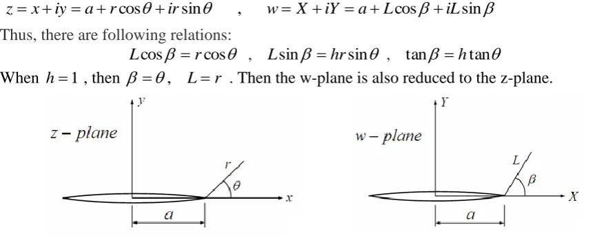
For the crack problem, rectangular and polar coordinates are shown in Figure 1. The polar coordinate system centered at the crack tip may be adequate for local stress analysis. In terms of the polar coordinates (in z-plane and w-plane), the complex variables can be written as:
sin , cos sin
cos ir w X iY a L iL
r a iy x
z (6)
Thus, there are following relations: cos
cos r
L , Lsin hrsin , tan htan
[image:2.595.69.501.524.697.2]When h1 , then , Lr . Then the w-plane is also reduced to the z-plane.
Figure 1. Scheme of the coordinates in z-plane and w-plane.
Consider an analytic function of complex variable, (w), and it can be expressed as:
) , ( ) , ( Im
Re )
(w i PiQP x y iQ x y
) ( 1 Im Re 1 1 Im Re y Q i y P h Y Q i Y P i i y w dw d h y h Y X Q i X P x Q i x P i x w dw d x X (8)
Obviously, it is easy to derive the following differential equation:
x Q X Q y P h Y P y Q h Y Q x P X P 1 , 1 (9)
Which can be written as follows:
0 1 , 0 1 2 2 2 2 2 2 2 2 2 2 2 2 2 2 2 2 2 2 y Q h x Q Y Q X Q y P h x P Y P X P (10)
Therefore, two functions P and Q are harmonic functions in w-plane.
The Airy stress function U can be expressed by the real function, P(x,y) or Q(x,y). Consider an infinite plane with the crack along the x-axis shown in Figure 1, and consider the problem of Mode II loading. The Airy stress function can be determined by the form:
AyP Ay
U Re (11)
Where, A is a real constant. The derivatives of U with respect to x or y are given by:
2 2 2 2 2 2 2 2 2 2 2 , , , y P Ay y P A y U y x P Ay x P A y x U x P Ay x U y P Ay AP y U x P Ay x U (12) On the basis of above equations, then Equation (5) becomes:
0 ) ( 4 ] 2 [ 2 3 2 4 4 2 4 y x P B h x P y C B h h (13) Where, 2 1 12 12 1 , 2 E E C G E
B . Thus the solution must be followed by the characteristic
equations, and also reduced to:
0 ,
0
2 2 2
4
B h C
Bh
h (14)
The solution of the characteristic equation (14) is given as:
2 1 12 12 1 2 2 E E G E C B
h
(15)
So the positive real root can be obtained, that is:
4 2 1 12 12 1 2 E E G E
h
(16)
y x
P Ay x P A x
P Ay y
P Ay y P
A y xy
x
2 22 , 22 , 2
(17)
Define (w), thus (w) . Then by Eq. (8), some relations are given as:
Im Im
, Re
Re h h
y P x
P
Im ,
Re ,
Re
2 2
2 2
2 2
h y x
P h
y P x
P
Therefore, the stresses can be reduced to:
2AhIm Ah2yRe , y AyRe , xy ARe AhyIm
x
(18)
Evidently, the analytic function can be as a new usual stress function.
Solution of Stresses
For Mode II crack problem, the plate with a line crack is subjected to uniform shear loading ~ at infinity. Consider the following stress boundary conditions:
0
xy
y
at x a and y0 (free crack surfaces) (19)
0
y
x
,
~
xy at
2 2
y
x (20)
In order for the stress function to meet the preceding boundary value problem, the complex function can be selected as:
2 2
a w
w
(21)
Substituting the stress function Eq. (21) into Eq. (18), and also using the boundary conditions Eqs. (19) and (20), the coefficients A can be derived as: A~. The stresses can be determined as follows:
] ) (
Im [Re
~ ] Im [Re
~
) (
Re ~ Re
~
] ) (
Re 2
[Im ~ ] Re Im
2 [ ~
2 / 3 2 2
2
2 2 2 / 3 2 2
2
2 / 3 2 2
2 2
2 2 2
a w
hy a
a w
w hy
a w
y a y
a w
y h a
a w
hw y
h h
xy y x
(22) In the vicinity of the crack tip (ra), the functions in Eq. (22) can be simplified as:
) exp( 2
) )( (
2
2
i aL a
w a w a
w , )
2 exp( 2 ) exp( 2
2 2
L i
a
i aL
a
a w
w
) 3 exp( sin
sin
2
2
i a
L a hy
a
) 2 3 sin 2 sin 1 ( 2 cos 2 ) 2 3 sin 2 sin 2 (cos 2
2 3 cos 2 cos 2 sin 1
2 2 3 cos 2 sin
2
) 2 3 cos 2 cos 2 ( 2 sin 2 )
2 3 cos 2 sin 2
sin 2 ( 2
L K
L K
h L K h
L K
h L K h
h L K
II II
xy
II II
y
II II
x
(23) For the isotropic materials (h1, then , Lr), the stresses can be derived as:
) 2 3 sin 2 sin 1 ( 2 cos 2
2 3 cos 2 cos 2 sin 2
) 2 3 cos 2 cos 2 ( 2 sin 2
r K
r K
r K
II xy
II y
II x
(24) Obviously, the stress fields in w-plane for the orthotropic material are similar to that of the isotropic material. Nevertheless, the stress coefficients are not quate the same.
Acknowledgements
This research was financially supported by the National Science Foundation of China (51475372).
References
[1] G.C. Sih: Mechanics of fracture initiation and propagation. Kluwer Academic Publishers, (1991).
[2] C.T. Sun: Fracture mechanics. Elsevier Inc., (2012).
[3] M. Fakoor, N.M. Khansari. Mixed mode I/II fracture criterion for orthotropic materials based on damage zone properties. Eng Fract Mech 2016; 153: 407-420.